# HSL-4XMO

High Speed Link

4-Axis Motion Control Module

User's Manual

Manual Rev. 2.01

Revision Date: May 31, 2005

Part No: 50-11001-2010

![The image displays the universal recycling symbol set against a solid black circular background. Three white arrows are arranged in a continuous triangular loop, each arrow detailed with three parallel lines running along its shaft.](.hsl-4xmo-manual-8/958170f82abd6f3274e6d11a29820187c2a486c80dca270514d4d6396dab9e74.jpg)
Recycled Paper

Copyright 2005 ADLINK TECHNOLOGY INC.

All Rights Reserved.

The information in this document is subject to change without prior notice in order to improve reliability, design, and function and does not represent a commitment on the part of the manufacturer.

In no event will the manufacturer be liable for direct, indirect, special, incidental, or consequential damages arising out of the use or inability to use the product or documentation, even if advised of the possibility of such damages.

This document contains proprietary information protected by copyright. All rights are reserved. No part of this manual may be reproduced by any mechanical, electronic, or other means in any form without prior written permission of the manufacturer.

# Trademarks

Product names mentioned herein are used for identification purposes only and may be trademarks and/or registered trademarks of their respective companies.

# Getting Service from ADLINK

Customer Satisfaction is top priority for ADLINK Technology Inc. Please contact us should you require any service or assistance.

# ADLINK TECHNOLOGY INC.

Web Site: http://www.adlinktech.com

Sales & Service: Service@adlinktech.com

TEL: +886-2-82265877

FAX: +886-2-82265717

Address: 9F, No. 166, Jian Yi Road, Chungho City,

Taipei, 235 Taiwan

Please email or FAX this completed service form for prompt and satisfactory service.

<table><tr><td colspan="2">Company Information</td></tr><tr><td>Company/Organization</td><td></td></tr><tr><td>Contact Person</td><td></td></tr><tr><td>E-mail Address</td><td></td></tr><tr><td>Address</td><td></td></tr><tr><td>Country</td><td></td></tr><tr><td>TEL</td><td>FAX:</td></tr><tr><td>Web Site</td><td></td></tr><tr><td colspan="2">Product Information</td></tr><tr><td>Product Model</td><td></td></tr><tr><td>Environment</td><td>OS:M/B: CPU:Chipset: Bios:</td></tr></table>

Please give a detailed description of the problem(s):

# Table of Contents

# Table of Contents...... i

# List of Tables...... iv

# List of Figures ...... v

# 1 Introduction ...... 1

1.1 Features.... 2
1.2 Specifications.... 3
1.3 Supported Software 5

Programming Library 5

Motion Creator on LinkMaster Utility 5

# 2 Installation 7

2.1 Package Contents 7
2.2 HSL-4XMO-CG-N/P Mechanical Drawing 8
2.3 HSL-4XMO-CD-N/P Mechanical Drawing 9
2.4 CN1 Pin Assignments: External Power Input 10
2.5 CN2 Pin Assignment: Emergency Input and General Input Common.... 10
2.6 HS1,2 Pin Assignments: HSL Communication Signal (RJ-45).
11
2.7 HS3 Pin Assignments: HSL Communication Signal (WAGO Type) 11
2.8 CM1-CM4 Pin Assignments: For HSL-4XMO-CG-N/P ..... 11
2.9 CM1-CM4 Pin Assignments: For HSL-4XMO-CD-N/P ..... 13
2.10 IOIF1-4 Pin Assignments: Mechanical I/O and GPIO Signal Connector.... 13
2.11 S1: Switch Setting for HSL Slave ID 14
2.12 JP1: Jumper Setting for HSL Communication Speed Selection 14
2.13 JP2 - 3: Jumper Setting for HSL Transmission Mode...... 15
2.14 JP4: Jumper Setting for HSL Termination Resistor 15
2.15 JP5-8, JP10-13: Enable/Disable DO to reset servo driver. 16
2.16 JP9: NPN/PNP setting of EMG signal 16

# 3 Signal Connections.... 17

3.1 Pulse Output Signals OUT and DIR 18

3.2 Encoder Feedback Signals EA, EB and EZ.... 20

3.3 Origin Signal ORG 22

3.4 End-Limit Signals PEL and MEL 23

3.5 Ramping-down & Position Latch 23

3.6 In-position Signal INP 24

3.7 Alarm Signal ALM 25

3.8 Deviation Counter Clear Signal (ERC).... 25

3.9 General-purpose Signal SVON 26

3.10 General-purpose Signal RDY 26

3.11 Position Compare Output CMP 27

3.12 Emergency Stop Input EMG 27

3.13 General-purpose Input 28

3.14 General-purpose Output 28

# 4 Operation Theory.... 31

4.1 Communication Block Diagram.... 31

4.2 Host Command 31

4.3 Command Delivering Time 32

4.4 Command Dispatching in DSP 34

4.5 The role of DSP and motion ASIC 35

4.6 Motion Control Modes 35

Pulse Command Output 35

Velocity Mode Motion 37

Trapezoidal Motion 38

S-curve Profile Motion 41

Linear interpolation for 2-4 axes 44

Circular interpolation for 2 axes 48

Circular Interpolation with Acc/dec Time 49

Relationship between Velocity and Acceleration Time . 50

Home Return Mode 53

4.7 The Motor Driver Interface 63

INP 63

ALM 64

ERC 64

SVON and RDY 65

4.8 The Limit Switch Interface and I/O Status.... 66

SD/LTC 66

EL 67

ORG 67

4.9 The Counters 68

Command Position Counter 68

Feedback Position Counter 69

Position Error Counter 71

General Purpose Counter 71

Target Position Recorder 72

4.10 Multiple HSL-4XMO Operations 73

4.11 Change Position Or Speed On The Fly 74

Change Speed on the Fly 74

Change Position on the Fly 80

4.12 Position Compare 82

Comparators of the HSL-4XMO 82

Position Compare 83

4.13 Backlash Compensator and Vibration Suppression ..... 86

4.14 Software Limit Function 87

4.15 Point Table Management.... 87

4.16 Motion Script Download 88

# 5 Motion Creator in LinkMaster.... 89

5.1 Execute Motion Creator in LinkMaster 89

5.2 About Motion Creator in LinkMaster 89

5.3 Motion Creator Form Introducing.... 91

Main Menu 91

Interface I/O Configuration Menu 92

Pulse IO Configuration Menu 93

Operation Menu 95

# 6 Appendix.... 103

6.1 HSL-4XMO Command Execution Time 103

# Warranty Policy.... 105

# List of Tables

Table 2-1: CN1 Pin Assignments: External Power Input ..... 10

Table 2-2: CN2 Pin Assignments: Emergency Input and General Input Common 10

Table 2-3: HS1-HS2 Pin Assignments: HSL Communication Signal (RJ-45) 11

Table 2-4: HS3 Pin Assignments: HSL Communication Signal (WAGO type) 11

Table 2-5: CM1-CM4 Pin Assignments: Servo Interface ..... 11

Table 2-6: CM1-CM4 Pin Assignments: For HSL-4XMO-CD-N/P 13

Table 2-7: IOIF1-4 Pin Assignments: Mechanical I/O and GPIO Signal Connector 13

Table 3-1: Encoder Power / External Resistor 21

Table 4-1: Base Scan Times 33

Table 4-2: Pulse Command Output 35

Table 4-3: Single Axis Motion Functions 44

Table 4-4: Counter Summary 72

Table 4-5: Multiple HSL-4XMO Operations 73

Table 4-6: HSL\_M\_v\_change() Example 77

Table 4-7: HSL\_M\_p\_change() Constraints 82

Table 4-8: HSL-4XMO Comparators 82

Table 6-1: Command Executuation Classifications ...... 103

Table 6-2: HSL-4XMO Command Execution Times ..... 103

# List of Figures

Figure 2-1: HSL-4XMO-CG-N/P Mechanical Drawing 8

Figure 2-2: HSL-4XMO-CD-N/P Mechanical Drawing 9

Figure 2-3: S1: Switch Setting for HSL Slave ID.... 14

Figure 2-4: JP1: HSL Communication Speed Selection Jumper Setting.... 14

Figure 2-5: JP2 - 3: Jumper Setting for HSL Transmission Mode 15

Figure 2-6: JP4: HSL Termination Resistor Jumper Setting ..... 15

Figure 2-7: JP5-8, JP10-13: Enable/Disable DO to reset servo driver 16

Figure 2-8: JP9: NPN/PNP setting of EMG signal 16

Figure 3-1: OUT and DIR Signals on the 4 Axes 18

Figure 3-2: Non-differential Type Wiring Example 19

Figure 3-3: EA, EB, and EZ signals 20

Figure 3-4: Connection to Line Driver Output 21

Figure 3-5: Connection to Open Collector Output.... 22

Figure 3-6: Origin Signal ORG 22

Figure 3-7: End-Limit Signals PEL and MEL 23

Figure 3-8: Ramping-down & Position Latch 24

Figure 3-9: In-position Signal INP 24

Figure 3-10: Alarm Signal ALM 25

Figure 3-11: Deviation Counter Clear Signal (ERC) 26

Figure 3-12: General-purpose Signal SVON 26

Figure 3-13: General-purpose Signal RDY 27

Figure 3-14: Position Compare Output CMP 27

Figure 3-15: Emergency Stop Input EMG 28

Figure 3-16: General-purpose Input.... 28

Figure 3-17: NPN Type General Purpose Output 29

Figure 3-18: PNP Type General Purpose Output 29

Figure 4-1: Communication Block Diagram 31

Figure 4-2: Single Command Timing 33

Figure 4-3: DSP Multi-Tasks 34

Figure 4-4: Single Pulse Output Mode (OUT/DIR Mode)...... 36

Figure 4-5: Dual Pulse Output Mode (CW/CCW Mode) ...... 37

Figure 4-6: Velocity Mode Motion 38

Figure 4-7: Trapezoidal Motion 39

Figure 4-8: Encoder Diagram.... 41

Figure 4-9: S-curve Profile Motion 42

Figure 4-10: Automatic Velocity Decrease.... 43

Figure 4-11: 2 Axes Linear Interpolation.... 45

Figure 4-12: 3-Axis Linear Interpolation.... 46

Figure 4-13: Circular interpolation for 2 axes.... 48

Figure 4-14: Circular Interpolation with Acc/dec Time .... 50

Figure 4-15: Velocity and Acceleration Time A.... 51

Figure 4-16: Velocity and Acceleration Time B 52

Figure 4-17: home\_mode=0....54

Figure 4-18: home\_mode=1....55

Figure 4-19: home\_mode=3....55

Figure 4-20: home\_mode=4....56

Figure 4-21: home\_mode=5.... 57

Figure 4-22: home\_mode=6....57

Figure 4-23: home\_mode=7....57

Figure 4-24: home\_mode=8....58

Figure 4-25: home\_mode=9.... 58

Figure 4-26: home\_mode=10....59

Figure 4-27: home\_mode=11....60

Figure 4-28: home\_mode=12....60

Figure 4-29: Home Search Example.... 61

Figure 4-30: 90° Phase Difference Signals....70

Figure 4-31: Change Speed on the Fly 74

Figure 4-32: HSL\_M\_v\_change() Theory.... 76

Figure 4-33: Velocity Suggestions A....77

Figure 4-34: Velocity Suggestions B 78

Figure 4-35: Velocity Example 78

Figure 4-36: Velocity Profile Example....79

Figure 4-37: Change Position on the Fly.... 80

Figure 4-38: Theory of HSL\_M\_p\_change() 81

Figure 4-39: Continuously Comparison with Trigger Output...... 84

Figure 4-40: Vibration Suppression.... 86

Figure 5-1: HSL Master Utility 90

Figure 5-2: Main Menu....91

Figure 5-3: Interface I/O Configuration Menu.... 92

Figure 5-4: Pulse IO Configuration Menu.... 94

Figure 5-5: Operation Menu 96

Figure 5-6: Show Velocity Curve.... 97

Figure 5-7: Home Mode Configuration.... 98

# 1 Introduction

The HSL-4XMO is a 4-axis motion controller module for HSL system. It can generate high frequency pulses (6.55MHz) to drive stepper or servomotors. As a motion controller, it can provide 2-axis circular interpolation, 4-axis linear interpolation, or continuous interpolation for continual velocity. Also, changing position/speed on the fly is available with a single axis operation.

Multiple HSL-4XMO modules can be used in one HSL system. Incremental encoder interface on all four axes provide the ability to correct positioning errors generated by inaccurate mechanical transmissions. With the aid of on board DSP, the HSL-4XMO can also perform many real-time applications without compromising CPU resources. In addition, a mechanical sensor interface, servo motor interface, and general-purposed I/O signals are provided for easy system integration.

The HSL-4XMO uses one ASIC (PCL6045) to perform all 4 axes motion controls and one DSP to communicate with Host PC and HSL protocol. The motion control functions include linear and S-curve acceleration/deceleration, circular interpolation between two axes, linear interpolation between 2\~4 axes, continuous motion positioning, and 13 home return modes. All these functions and complex computations are performed internally by the ASIC, thus limiting the impact on the PC's CPU usage. The DSP can perform as a motion path-loading manager without consuming Host PC's resource. It is more powerful than traditional ASIC-based motion control card.

# 1.1 Features

▶ High Speed Link (HSL) protocol compatible
▶ 3M/6M/12M data transfer rate selectable
▶ Support dual and half duplex modes
▶ On board DSP (TMS320C6711)
▶ 4-axis stepper or servo motor control by pulse signal command
▶ Maximum pulse output frequency: 6.55 MPPS
▶ Pulse output types: OUT/DIR (single pulse), CW/CCW (dual pulse)
▶ Support up to 63 axes in one HSL network
▶ Motion point table management
▶ Motion script download for precision timing motion control
▶ Any 2 of 4 axes circular interpolation in one module
▶ Any 2-4 of 4 axes linear interpolation in one module
▶ Continuous interpolation for contour following motion
▶ 3 Command buffers for special speed profile motion
▶ Change position and speed on the fly
▶ Change speed by condition comparing
▶ 13 home return modes with auto searching
▶ 2 ways software end-limits of each axis
▶ 28-bit up/down incremental encoder interface of each axis
▶ Dedicated motion I/O : home (DOG), index signal (EZ), end limit, servo on, INP, ERC, ALM, motion interface of each axis
▶ 4 general-purpose DI/DO channels
▶ One Emergency input with hardware motion stop function
▶ High-speed position counter latch input for each axis
▶ Continuous position compare with trigger pulse output of each axis
▶ All digital input and output signals are 2500Vrms isolated
▶ Includes Motion Creator, a Microsoft Windows-based application development software built in LinkMaster Utility

▶ User-friendly function libraries and utilities for DOS and Windows 9x/NT/2000/XP. Also supported under Linux

# 1.2 Specifications

# Command Response Time

▶ Half Duplex: 240us for one module under 6Mhz data transfer rate
▶ Full Duplex: 240us for two modules under 6Mhz data transfer rate

# Motion Control

▶ Maximum controllable axes in one module: 4
▶ Internal reference clock: 19.66MHz
▶ Position counter range: -134,217,728 to +134,217,727 (28-bit)
▶ Command counter setting range: -134,217,728 to +134,217,728 (28-bit)
▶ Pulse rate setting range: 1\~65,535 (16-bit)
▶ Pulse rate multiplier setting range: 0.1\~100

# Pulse Output

▶ Line driver output
▶ Max. Speed: 6.55 Mhz
▶ Output Voltage:

▷ Logic H: 2.5V min.
▷ Logic L: 0.5V max.

▶ Isolated voltage: 500Vrms

# Encoder Input

▶ Incremental Encoder Input
▶ Max. Speed: 5 Mhz
▶ Input Voltage:

▷ Logic H: 3\~5V
▷ Logic L: 0\~2.4V

▶ Input resistor: 220Ω @ 0.125W
▶ Isolated voltage: 500Vrms

# Digital Input

▶ Sink or source type can be selected via ICOM
▶ Switching capability: 10K Hz
▶ Input voltage range:

▷ Logic H: 14.4\~24V

▷ Logic L: 0\~5V

▶ Input resistor: 4.7KΩ @ 0.5W
▶ Isolated voltage: 500Vrms

# Digital Output

▶ Output type: Open-collector (PC3H7C)
▶ Sink Current: 4mA max.
▶ Switching capability: 10KHz @ 24V, load = 4.7KΩ
▶ Isolated voltage: 500Vrms

# General Purpose Output

▶ Output type: NPN sinking type for –N module; PNP sourcing type for –P module
▶ Sink Current: 90 mA max.
▶ Switching capability: 2 KHz @ 24V, load = 300Ω
▶ Isolated voltage: 500 Vrms

# General Specifications

▶ Operating Temperature: $0^{\circ}$ C – $60^{\circ}$ C
▶ Storage Temperature: $-20^{\circ}C - 80^{\circ}C$
▶ Humidity: 0% – 90%, non-condensing

# Power Consumption

▶ 5 Watts max. @ 24Vin

# Dimensions

▶ 163.5mm (W) × 74.9mm (D) × 52.7mm (H)

# 1.3 Supported Software

# Programming Library

The Library supports Borland C/C++ (Version: 3.1) and Windows 95/98/NT/2000/XP. These function libraries are shipped with the module. Users can check ADLINK website for latest update.

This module supports DOS/Windows 98/NT/2000/XP. For other OS, please contact the local vendors.

# Motion Creator on LinkMaster Utility

This Windows-based utility is used to setup cards, motors, and systems. It can also aid in debugging hardware and software problems. It allows users to set I/O logic parameters to be loaded in their own program. This product is also bundled with the card.

# 2 Installation

This chapter describes how to install the HSL-4XMO series. Please follow these steps below:

▶ Check what you have (section 2.1)
▶ Check the PCB (section 2.2)
▶ Install the hardware (section 2.3)
▶ Install the software driver (section 2.4)
▶ Understanding the I/O signal connections (chapter 3) and their operation (chapter 4)
▶ Understanding the connector pin assignments (the remaining sections) and wiring the connections

# 2.1 Package Contents

In addition to this User's Guide, the package also includes the following items:

▶ HSL-4XMO: Advanced 4-Axis Servo / Stepper Motion Control Card (HSL-4XMO-CG-N/P, HSL-4XMO-CD-N/P)
▶ ADLINK All-in-one Compact Disc

If any of these items are missing or damaged, contact the dealer from whom you purchased the product. Save the shipping materials and carton to ship or store the product in the future.

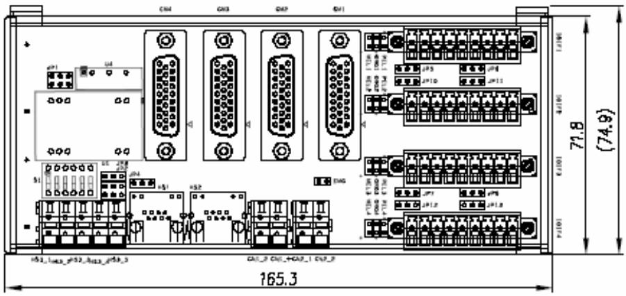
2.2 HSL-4XMO-CG-N/P Mechanical Drawing
![JP1\n3M\n6M\n12M\nS1\nJP3\nJP2\nJP4\nFD HO OFF ON\nFG T+ T- R+ R-\nHS1\nHS2 CM1\nEGND E24Y ICOM EWG\nHS3\nCM1\nCM2\nCM3\nCM4\nCELI* (W)\nOPG1\nPELI*\nMEI3 MELF\nOPG0 ONG\nPELI* (W)\nPELI* (W)\nADLINK\nTECHNOLOGY INC\nCE\nIOIF1\nIOIF2\nIOIF3\nIOIF4\n71.8\n(74.9)\n165.3](.hsl-4xmo-manual-8/4cabcfdfc00bb019ef0e34096e2833b6c9ee5b6e66c1ab60062cffd6d4d4ee28.jpg)

![52.7](.hsl-4xmo-manual-8/b3c9b760f430790cef04250a1a4bfc4c8268777b74fbb8cc7208163132768c4f.jpg)

Figure 2-1: HSL-4XMO-CG-N/P Mechanical Drawing

<table><tr><td>CN1:</td><td>External Power Input Connector (+24V)</td></tr><tr><td>CN2:</td><td>Digital Input Common and Emergency Input Pin</td></tr><tr><td>HS1-2:</td><td>HSL Communication Signal Connector (RJ45)</td></tr><tr><td>HS3:</td><td>HSL Communication Signal Connector (WAGO)</td></tr><tr><td>CM1-4:</td><td>Servo Interface Signal Connector</td></tr><tr><td>IOIF1-4:</td><td>Mechanical I/O and GPIO Signal Connector</td></tr><tr><td>S1:</td><td>Slave ID Switch</td></tr><tr><td>JP1:</td><td>Communication Speed Selection Jumper</td></tr><tr><td>JP2-3:</td><td>Full Duplex / Half Duplex Selection Jumper</td></tr><tr><td>JP4:</td><td>HSL Termination Resistor Jumper</td></tr></table>

# 2.3 HSL-4XMO-CD-N/P Mechanical Drawing

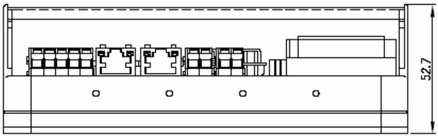
![CN4\nCN3\nCN2\nCN1\nU4\nJP1\nJP2\nJP3\nJP4\nJP5\nJP6\nJP7\nJP8\nJP9\nJP10\nJP11\nJP12\nJP13\nJP14\nJP15\nJP16\nJP17\nJP18\nJP19\nJP20\nJP21\nJP22\nJP23\nJP24\nJP25\nJP26\nJP27\nJP28\nJP29\nJP30\nJP31\nJP32\nJP33\nJP34\nJP35\nJP36\nJP37\nJP38\nJP39\nJP40\nJP41\nJP42\nJP43\nJP44\nJP45\nJP46\nJP47\nJP48\nJP49\nJP50\nJP51\nJP52\nJP53\nJP54\nJP55\nJP56\nJP57\nJP58\nJP59\nJP60\nJP61\nJP62\nJP63\nJP64\nJP65\nJP66\nJP67\nJP68\nJP69\nJP70\nJP71\nJP72\nJP73\nJP74\nJP75\nJP76\nJP77\nJP78\nJP79\nJP80\nJP81\nJP82\nJP83\nJP84\nJP85\nJP86\nJP87\nJP88\nJP89\nJP90\nJP91\nJP92\nJP93\nJP94\nJP95\nJP96\nJP97\nJP98\nJP99\nJP100\nJP101\nJP102 (74.9)\n71.8](.hsl-4xmo-manual-8/4bbb58e0ac609d0814511cc52633b64d185a9048fc3867677d427bf9a84b3aa8.jpg)

![Technical line drawing of an electronic device rear panel with internal components and a dimension label (52.7) — no readable text or symbols beyond the dimension line.](.hsl-4xmo-manual-8/c781fb3b90f5c2899ed647fe6a8b0e6dca6d75c3b66afbf58f409631f908a0e3.jpg)

Figure 2-2: HSL-4XMO-CD-N/P Mechanical Drawing

<table><tr><td>CN1:</td><td>External Power Input Connector (+24V)</td></tr><tr><td>CN2:</td><td>Digital Input Common and Emergency Input Pin</td></tr><tr><td>HS1-2:</td><td>HSL Communication Signal Connector (RJ45)</td></tr><tr><td>HS3:</td><td>HSL Communication Signal Connector (WAGO)</td></tr><tr><td>CM1-4:</td><td>Servo Interface Signal Connector</td></tr><tr><td>IOIF1-4:</td><td>Mechanical I/O and GPIO Signal Connector</td></tr><tr><td>S1:</td><td>Slave ID Switch</td></tr><tr><td>JP1:</td><td>Communication Speed Selection Jumper</td></tr><tr><td>JP2-3:</td><td>Full Duplex/Half Duplex Jumper</td></tr><tr><td>JP4:</td><td>Termination Resistor Jumper</td></tr><tr><td>JP5-8:</td><td>Enable/Disable DO to reset servo driver</td></tr><tr><td>JP9:</td><td>NPN/PNP setting of EMG signal</td></tr><tr><td>JP10-13:</td><td>NPN/PNP setting of DO signal</td></tr></table>

# 2.4 CN1 Pin Assignments: External Power Input

<table><tr><td>CN1 Pin Name</td><td>Description</td></tr><tr><td>EGND</td><td>External power ground</td></tr><tr><td>E24V</td><td>+24VDC ±5% External power supply</td></tr></table>

Table 2-1: CN1 Pin Assignments: External Power Input

# 2.5 CN2 Pin Assignment: Emergency Input and General Input Common

<table><tr><td>CN2 Pin Name</td><td>Description</td></tr><tr><td>ICOM</td><td>Mechanical Input and General Input Common</td></tr><tr><td>EMG</td><td>Emergency Stop Input</td></tr></table>

Table 2-2: CN2 Pin Assignments: Emergency Input and General Input Common
Note: ICOM should be connected to either EGND or E24V

# 2.6 HS1,2 Pin Assignments: HSL Communication Signal (RJ-45).

![Pure electrical circuit lines without any symbols](.hsl-4xmo-manual-8/1d0ab258dac878605090ceb12a5a5666dfc92f786fa3559d90b811920a926f01.jpg)

8 1

RJ45 Female Connector

<table><tr><td>PIN NO.</td><td>PIN OUT</td></tr><tr><td>PIN 1</td><td>NC</td></tr><tr><td>PIN 2</td><td>NC</td></tr><tr><td>PIN 3</td><td>TXD+</td></tr><tr><td>PIN 4</td><td>RXD-</td></tr><tr><td>PIN 5</td><td>RXD+</td></tr><tr><td>PIN 6</td><td>TXD-</td></tr><tr><td>PIN 7</td><td>NC</td></tr><tr><td>PIN 8</td><td>NC</td></tr></table>

Table 2-3: HS1-HS2 Pin Assignments: HSL Communication Signal (RJ-45)

# 2.7 HS3 Pin Assignments: HSL Communication Signal (WAGO Type)

<table><tr><td>HS3 Pin Name</td><td>Description</td></tr><tr><td>FG</td><td>Shielding ground</td></tr><tr><td>T+</td><td>TXD+</td></tr><tr><td>T-</td><td>TXD-</td></tr><tr><td>R+</td><td>RXD+</td></tr><tr><td>R-</td><td>RXD-</td></tr></table>

Table 2-4: HS3 Pin Assignments: HSL Communication Signal (WAGO type)

# 2.8 CM1-CM4 Pin Assignments: For HSL-4XMO-CGN/P

<table><tr><td>No.</td><td>Name</td><td>Function</td><td>No.</td><td>Name</td><td>Function</td></tr><tr><td>1</td><td>EA+</td><td>Encoder A-phase (+)</td><td>2</td><td>EA-</td><td>Encoder A-phase (-)</td></tr><tr><td>3</td><td>EB+</td><td>Encoder B-phase (+)</td><td>4</td><td>EB-</td><td>Encoder B-phase (-)</td></tr><tr><td>5</td><td>EZ+</td><td>Encoder Z-phase (+)</td><td>6</td><td>EZ-</td><td>Encoder Z-phase (-)</td></tr><tr><td>7</td><td>PGND</td><td>Ground of pulse I/O signals</td><td>8</td><td>PGND</td><td>Ground of pulse I/O signals</td></tr></table>

Table 2-5: CM1-CM4 Pin Assignments: Servo Interface

<table><tr><td>No.</td><td>Name</td><td>Function</td><td>No.</td><td>Name</td><td>Function</td></tr><tr><td>9</td><td>OUT+</td><td>Pulse signal (+)</td><td>10</td><td>OUT-</td><td>Pulse signal (-)</td></tr><tr><td>11</td><td>DIR+</td><td>Direction signal (+)</td><td>12</td><td>DIR-</td><td>Direction signal (-)</td></tr><tr><td>13</td><td>EGND</td><td>Ext. power ground</td><td>14</td><td>SVON</td><td>Servo on output signal</td></tr><tr><td>15</td><td>INP</td><td>In-position input signal</td><td>16</td><td>ERC</td><td>Deviation counter clear output signal</td></tr><tr><td>17</td><td>EGND</td><td>External power ground</td><td>18</td><td>E24V</td><td>External power supply, +24V</td></tr><tr><td>19</td><td>RDY</td><td>Ready input signal</td><td>20</td><td>ALM</td><td>Alarm input signal</td></tr></table>

Table 2-5: CM1-CM4 Pin Assignments: Servo Interface

# 2.9 CM1-CM4 Pin Assignments: For HSL-4XMO-CD-N/P

<table><tr><td>No.</td><td>Name</td><td>Function</td><td>No.</td><td>Name</td><td>Function</td></tr><tr><td>1</td><td>SVON</td><td>Servo on output signal</td><td>2</td><td>INP</td><td>In-position input signal</td></tr><tr><td>3</td><td>ERC</td><td>Deviation counter clear output signal</td><td>4</td><td>RDY</td><td>Ready input signal</td></tr><tr><td>5</td><td>OUT-</td><td>Pulse signal (-)</td><td>6</td><td>OUT+</td><td>Pulse signal (+)</td></tr><tr><td>7</td><td>EA-</td><td>Encoder A-phase (-)</td><td>8</td><td>EA+</td><td>Encoder A-phase (+)</td></tr><tr><td>9</td><td>N.C.</td><td>Not Connected</td><td>10</td><td>RST</td><td>Alarm reset output signal</td></tr><tr><td>11</td><td>ALM</td><td>Alarm input signal</td><td>12</td><td>E24V</td><td>External power supply, +24V</td></tr><tr><td>13</td><td>EGND</td><td>Ext. power ground</td><td>14</td><td>N.C.</td><td>Not Connected</td></tr><tr><td>15</td><td>PGND</td><td>Ground of pulse I/O signals</td><td>16</td><td>EB-</td><td>Encoder B-phase (-)</td></tr><tr><td>17</td><td>EB+</td><td>Encoder B-phase (+)</td><td>18</td><td>PGND</td><td>Ground of pulse I/O signals</td></tr><tr><td>19</td><td>EMG</td><td>Emergency stop output signal</td><td>20</td><td>EGND</td><td>External power ground</td></tr><tr><td>21</td><td>EGND</td><td>External power ground</td><td>22</td><td>EGND</td><td>External power ground</td></tr><tr><td>23</td><td>DIR-</td><td>Direction signal (-)</td><td>24</td><td>DIR+</td><td>Direction signal (+)</td></tr><tr><td>25</td><td>EZ-</td><td>Encoder Z-phase (-)</td><td>26</td><td>EZ+</td><td>Direction signal (+)</td></tr></table>

Table 2-6: CM1-CM4 Pin Assignments: For HSL-4XMO-CD-N/P

# 2.10 IOIF1-4 Pin Assignments: Mechanical I/O and GPIO Signal Connector

<table><tr><td>Pin No.</td><td>Pin Name</td><td>Description</td></tr><tr><td>1</td><td>E24V</td><td>External power supply, +24V</td></tr><tr><td>2</td><td>MEL</td><td>End limit input signal (-)</td></tr><tr><td>3</td><td>ORG</td><td>Origin input signal</td></tr><tr><td>4</td><td>PEL</td><td>End limit input signal (+)</td></tr><tr><td>5</td><td>LTC/SD</td><td>Ramp-down/position latch input signal (default for LTC)</td></tr><tr><td>6</td><td>DI/EZ</td><td>General purposed input/Index Input</td></tr><tr><td>7</td><td>DO</td><td>General purposed output</td></tr><tr><td>8</td><td>CMP</td><td>Position compare output</td></tr><tr><td>9</td><td>EGND</td><td>External power ground</td></tr></table>

Table 2-7: IOIF1-4 Pin Assignments: Mechanical I/O and GPIO Signal Connector

# 2.11 S1: Switch Setting for HSL Slave ID

![ON\n1 2 3 4 5 6](.hsl-4xmo-manual-8/3c1c9f13a831969024950b89b0d681973b5101e3cd49f0f6bb7c90662b5aa2a6.jpg)

![ON = 1\n100000 Start Address 1(1)\n010000 Start Address 2\n... ... \n... ... \n001111 Start Address 60\n101111 Not used\n011111 Not used\n111111 Not used\nOFF = 0](.hsl-4xmo-manual-8/7f58c72a4b96a36e5e2dadd2b59d6ff25cadb50f602ae17459ee5c0c098ee938.jpg)

Figure 2-3: S1: Switch Setting for HSL Slave ID

Note: Each HSL-4XMO occupies 4 HSL IDs. If using half duplex mode, the occupied ID will be continuously from this setting. For example, if you set the ID=1 then the occupied IDs will be 1, 2, 3, 4. If using full duplex mode, the occupied ID will be two ID steps in order. For example, if you set the ID=1 then the occupied IDs will be 1, 3, 5, 7.

# 2.12 JP1: Jumper Setting for HSL Communication Speed Selection

![JP1\n3M ○ ○\n6M ● ●\n12M ○ ○\n6 Mbps (default)](.hsl-4xmo-manual-8/8ae0d60ee511a1c8682d857a10c7e9e5e56beef4a58c19fede5943a596c6b74b.jpg)

Figure 2-4: JP1: HSL Communication Speed Selection Jumper Setting

# 2.13 JP2 - 3: Jumper Setting for HSL Transmission Mode

![JP3\nFull Duplex (Default)\nJP2\nFD HD\nJP3\nHalf Duplex\nJP2\nFD HD](.hsl-4xmo-manual-8/5bfadbf8c4a57fcd0280545801661919f3e6bc3fda0c80d7eb716722a68fab05.jpg)

Figure 2-5: JP2 - 3: Jumper Setting for HSL Transmission Mode

# 2.14 JP4: Jumper Setting for HSL Termination Resistor

![OFF ON\nDisable termination resistor\nOFF ON\nEnable termination resistor](.hsl-4xmo-manual-8/91a27e27be78671974778ea4bdbf43e9d95c1b00d693a4ef9023f8d34dc32927.jpg)

Figure 2-6: JP4: HSL Termination Resistor Jumper Setting

# 2.15 JP5-8, JP10-13: Enable/Disable DO to reset servo driver

![ALM_RSTx\nJP5-8 ○ ○ JP10-13\nNPN ○ ○ ○ PNP\nClosed: Enable alarm reset (default)\nOpen: Disable alarm reset\nNPN: The GPO of this module is NPN type (default)\nPNP: The GPO of this module is PNP type](.hsl-4xmo-manual-8/a01bcaea0bcffdc92f79f012ce4cd10e2edab831ed330684cb7d517ff435df2f.jpg)

Figure 2-7: JP5-8, JP10-13: Enable/Disable DO to reset servo driver

# 2.16 JP9: NPN/PNP setting of EMG signal

![JP9\nNPN ○ ○ ○\nPNP](.hsl-4xmo-manual-8/a63f939a1672def3293b1bce3641dd6bfe80d3230282b063e23cee225e481318.jpg)

NPN: The EMG signal is from NPN type sensor (default)

PNP: The EMG signal is from
PNP type sensor

Figure 2-8: JP9: NPN/PNP setting of EMG signal

# 3 Signal Connections

Signal connections of all I/O's are described in this chapter. Refer to the contents of this chapter before wiring any cables between the HSL-4XMO and any motor drivers.

This chapter contains the following sections:

▶ Section 3.1 Pulse Output Signals OUT and DIR
▶ Section 3.2 Encoder Feedback Signals EA, EB and EZ
▶ Section 3.3 Origin Signal ORG
▶ Section 3.4 End-Limit Signals PEL and MEL
▶ Section 3.5 Ramping-down & Position latch signals
▶ Section 3.6 In-position signals INP
▶ Section 3.7 Alarm signal ALM
▶ Section 3.8 Deviation counter clear signal ERC
▶ Section 3.9 General-purpose signals SVON
▶ Section 3.10 General-purpose signal RDY
▶ Section 3.11 Position compare output pin: CMP
▶ Section 3.12 General-purpose DI
▶ Section 3.13 General-purpose DO

# 3.1 Pulse Output Signals OUT and DIR

There are 4 axis pulse output signals on the HSL-4XMO. For each axis, two pairs of OUT and DIR signals are used to transmit the pulse train and to indicate the direction. The OUT and DIR signals can also be programmed as CW and CCW signal pairs. In this section, the electrical characteristics of the OUT and DIR signals are detailed. Each signal consists of a pair of differential signals. For example, OUT2 consists of OUT2+ and OUT2- signals.

The following wiring diagram is for OUT and DIR signals on the 4 axes.

![Based on the provided circuit diagram, here is the accurate description of the labeled blocks and their connections:\n\n**Labeled Blocks and Components:**\n*   **VCC** (Power supply input)\n*   **R** (Resistor)\n*   **OUT/DIR** (Input signal line)\n*   **2A** (Text label next to a diode symbol inside the first box)\n*   **2631** (Label for the main driver block)\n*   **VDD** (Power supply input)\n*   **OUT+, DIR+** (Output pin label)\n*   **OUT-, DIR-** (Output pin label)\n*   **PGND** (Power Ground label)\n\n**Connections:**\n*   **VCC** connects to one end of resistor **R**.\n*   The other end of resistor **R** connects to a junction.\n*   The input line **OUT/DIR** connects to the same junction.\n*   This junction connects to the input of a rectangular box containing a diode and an inverter.\n*   The output of this rectangular box connects to the input of the triangular block labeled **2631**.\n*   The block **2631** connects to **VDD** at the top.\n*   The block **2631** has outputs on the right side connecting to the labels **OUT+, DIR+** and **OUT-, DIR-**.\n*   The block **2631** connects to the **PGND** line at the bottom.\n*   A vertical dotted line separates the internal circuit components from the external output labels on the right.](.hsl-4xmo-manual-8/6a170421f6145e85a13b87f1a1a4dbee68456a0165ae26efe6cfc4e6d497856a.jpg)

Figure 3-1: OUT and DIR Signals on the 4 Axes

# Non-differential type wiring example:

Choose one of OUT/DIR+ and OUT/DIR- to connect to driver's OUT/DIR

![VDD\nInside Motion Controller\n2631\nOUT+, DIR+\nOUT-, DIR-\nFGND\nCOM\nR\nOUT/DIR\nInside Motor Driver\nGND](.hsl-4xmo-manual-8/b5cddf4ec83a370908ef8f3140613ddcd9508666f04c27fc3f7668d6938a77dd.jpg)

Figure 3-2: Non-differential Type Wiring Example

Warning: The sink current must not exceed 20mA or the 2631 will be damaged!

# 3.2 Encoder Feedback Signals EA, EB and EZ

The encoder feedback signals include EA, EB, and EZ. Every axis has six pins for three differential pairs of phase-A (EA), phase-B (EB), and index (EZ) inputs. EA and EB are used for position counting, and EZ is used for zero position indexing.

The input circuit of the EA, EB, and EZ signals is shown as follows:

![Inside HSL-4XMO\nPCL6045\nEA, EB\nEZ\nR\nEA+, EB+, EZ+\nEA-, EB-\nEZ-](.hsl-4xmo-manual-8/46715fcb2e88243dca36610303400dc6951bebf9ac1b784ac493ad492539b088.jpg)

Figure 3-3: EA, EB, and EZ signals

Please note that the voltage across each differential pair of encoder input signals (EA+, EA-), (EB+, EB-), and (EZ+, EZ-) should be at least 3.5V. Therefore, the output current must be observed when connecting to the encoder feedback or motor driver feedback as not to over drive the source. The differential signal pairs are converted to digital signals EA, EB, and EZ; then feed to the PCL6045 ASIC (R=220ohm).

Below are examples of connecting the input signals with an external circuit. The input circuit can be connected to an encoder or motor driver if it is equipped with: (1) a differential line driver or (2) an open collector output.

# Connection to Line Driver Output

To drive the HSL-4XMO encoder input, the driver output must provide at least 3.5V across the differential pairs with at least 6mA driving capacity. The grounds of both sides must be tied together. The maximum frequency will be 4Mhz or more depends on wiring distance and signal conditioning.

![PCI-\nHSL-\nEA+, EB+, EZ+\nEA-, EB-, EZ-\nPGND\nExternal Encoder / Driver\nWith line driver output\nA,B phase signals\nIndex signal\nGND](.hsl-4xmo-manual-8/b12c4e009ef3e67a633433929f4835999cb6f55228e9631306d956b2c815a69b.jpg)

Figure 3-4: Connection to Line Driver Output

# Connection to Open Collector Output

To connect with an open collector output, an external power supply is necessary. Some motor drivers can provide the power source. The connection between the HSL-4XMO, encoder, and the power supply is shown in the diagram below. Note that an external current limiting resistor R is necessary to protect the HSL-4XMO input circuit. The following table lists the suggested resistor values according to the encoder power supply.

<table><tr><td>Encoder Power (VDD)</td><td>External Resistor R</td></tr><tr><td>+5V</td><td>0Ω (None)</td></tr><tr><td>+12V</td><td>1.8kΩ</td></tr><tr><td>+24V</td><td>4.3kΩ</td></tr></table>

Table 3-1: Encoder Power / External Resistor

▶ $I_{f} = 6mA$ max.

![HSL-4XMO\nEA+, EB+, EZ+\nR\nVDD\nGND\nExternal Power for Encoder\nMotor Encoder / Driver\nWith Open Collector Output\nEA-, EB-, EZ-\nA, B phase signals\nIndex signal](.hsl-4xmo-manual-8/2e053422bf4bd3c34bc16cb4958dcc1580d4f6d4e83856bcee745a3e179f5f28.jpg)

Figure 3-5: Connection to Open Collector Output

For more operation information on the encoder feedback signals, refer to section 4.9.

# 3.3 Origin Signal ORG

The origin signals (ORG1-ORG4) are used as input signals for the origin of the mechanism.

The input circuit of the ORG signals is shown below. Usually, a limit switch is used to indicate the origin on one axis. The specifications of the limit switch should have contact capacity of +24V @ 6mA minimum. An internal filter circuit is used to filter out any high frequency spikes, which may cause errors in the operation.

![Filter Circuit\nTo PCL6045\nInside HSL-4XMO\nI=6mA Max.\n4.7K\nConnector\nICOM\nORG\n← Switch\nEGND](.hsl-4xmo-manual-8/82c1d7ec8b1ee15d868727d1528a5c37efde5622975eb3dcafc4111d3130b577.jpg)

Figure 3-6: Origin Signal ORG

When the motion controller is operated in the home return mode, the ORG signal is used to inhibit the control output signals (OUT and DIR). For detailed operations of the ORG signal, refer to section 4.8.

# 3.4 End-Limit Signals PEL and MEL

There are two end-limit signals PEL and MEL for each axis. PEL indicates the end limit signal is in the plus direction and MEL indicates the end limit signal is in the minus direction.

A circuit diagram is shown in the diagram below. The external limit switch should have a contact capacity of +24V @ 6mA minimum. Either 'A-type' (normal open) contact or 'B-type' (normal closed) contact switches can be used. The type of switch can be configured by software. For more details on EL operation, refer to section 4.8.

![Filter Circuit\nTo PCL6045\nInside HSL-4XMO\n4.7K\nI=6mA Max.\nConnector\nICOM\nPEL\nMEL\nSwitch\nEGND](.hsl-4xmo-manual-8/ebb2e485e3778e9c99a666a328b92b6ae1098e280e5692af2575c141d1d19e91.jpg)

Figure 3-7: End-Limit Signals PEL and MEL

# 3.5 Ramping-down & Position Latch

There is a SD/LTC signal for each of the 4 axes. A circuit diagram is shown below. Typically, the limit switch is used to generate a slow-down signal to drive motors operating at slower speeds. While act as the LTC signal, it will trigger the counter-value-capturing functions, which provides a precise position determination. For more details on SD/LTC operation, refer to section 4.8.

![Filter Circuit\nTo PCL6045\nInside HSL-4XMO\nI=6mA Max.\n4.7K\nConnector\nICOM\nSD/LTC\n← Switch\nEGND](.hsl-4xmo-manual-8/4a8125993ed593930bffb609d88796e43c81396d7bc3f90aed7565a31b400a17.jpg)

Figure 3-8: Ramping-down & Position Latch

# 3.6 In-position Signal INP

The in-position signal INP from a servo motor driver indicates its deviation error. If there is no deviation error then the servo's position indicates zero. The input circuit of the INP signals is shown in the diagram below:

![Inside HSL-4XMO\nE24V\nAxis\nTo PCL6045\n4.7K\nI=6mA Max.\nINP](.hsl-4xmo-manual-8/0170e935ae8da2ece9cff0a2aa294afdd4b479ec7a8dc844d5a82c3d5a2c8d86.jpg)

Figure 3-9: In-position Signal INP

The in-position signal is usually generated by the servomotor driver and is ordinarily an open collector output signal. An external circuit must provide at least 6mA current sink capabilities to drive the INP signal. For more details of INP signal operations, refer to section 4.7.

# 3.7 Alarm Signal ALM

The alarm signal ALM is used to indicate the alarm status from the servo driver. The input alarm circuit is shown below. The ALM signal usually is generated by the servomotor driver and is ordinarily an open collector output signal. An external circuit must provide at least 6mA current sink capabilities to drive the ALM signal. For more details of ALM signal operations, refer to section 4.7.

![Inside HSL-4XMO\nE24V\nTo PCL6045\n4.7K\nI=6mA Max.\nAXIS\nALM](.hsl-4xmo-manual-8/163f5a85430bb6baf4195e311d81e40c5cc2734392a4d591596eb4f8c183d48c.jpg)

Figure 3-10: Alarm Signal ALM

# 3.8 Deviation Counter Clear Signal (ERC)

The deviation counter clear signal (ERC) is active in the following 4 situations:

1. Home return is complete
2. End-limit switch is active
3. An alarm signal stops OUT and DIR signals
4. An emergency stop command is issued by software (operator)

The ERC signal is used to clear the deviation counter of the servo-motor driver. The ERC output circuit is an open collector with a maximum of 35V at 6mA driving capacity. For more details of ERC operation, refer to section 4.7.

![From PCL6045\nInside HSL-4XMO\n35V @ 6mA Maximum\nAXIS\nERC\nEGND](.hsl-4xmo-manual-8/e12ed8aeb26dfcd75cc8714b80c1e456a0d104431559fce0ef1b340881139e8b.jpg)

Figure 3-11: Deviation Counter Clear Signal (ERC)

# 3.9 General-purpose Signal SVON

The SVON signal can be used as a servomotor-on control or general- purposed output signal. The output circuit for the SVON signal is shown below:

![From PCL6045\nInside HSL-4XMO\n35V @ 6mA Maximum\nAXIS\nSVON\nEGND](.hsl-4xmo-manual-8/d6e8a0a9a430a88d3e749b8f02170315bfd1c142166196858ed3347c87b4462d.jpg)

Figure 3-12: General-purpose Signal SVON

# 3.10 General-purpose Signal RDY

The RDY signals can be used as motor driver ready input or general purpose input signals. The input circuit of RDY signal is shown in the following diagram:

![Inside HSL-4XMO\nE24V\nTo PCL6045\nI=6mA Max.\nRDY\nAXIS](.hsl-4xmo-manual-8/1d80a8ca602f9418f3737830d69726784d06711547520d3fc19cb0679d905b93.jpg)

Figure 3-13: General-purpose Signal RDY

# 3.11 Position Compare Output CMP

The HSL-4XMO provides 4 comparison output channels. The comparison output channel will generate a pulse signal when the encoder counter reaches a pre-set value set by the user.

The following wiring diagram is of the CMP signals:

![From PLD\nInside HSL-4XMO\n35V @ 6mA Maximum\nCMP\nEOGND\nIOIF](.hsl-4xmo-manual-8/b1c8445baca89713a45eb0d70409c38107a74f56787d00adc410f75c03270380.jpg)

Figure 3-14: Position Compare Output CMP

Note: CMP trigger type can be set as normal low (rising edge) or normal high (falling edge). Default setting is normal high.

# 3.12 Emergency Stop Input EMG

There is emergency stop input pin for this module. When EMG is active, all the motion pulse output command will be rejected until the EMG is deactive.

A circuit diagram is shown in the diagram below. The emergency stop switch should have a contact capacity of +24V @ 6mA minimum. Either ‘A-type’ (normal open) contact or ‘B-type’ (normal closed) contact switches can be used. The type of switch can be configured by software.

![Filter Circuit\nTo PCL6045\nInside HSL-4XMO\n4.7K\nI=6mA Max.\nConnector\nICOM\nBM\nG\nSwitch\nEGND](.hsl-4xmo-manual-8/ad3e4da35b7cd88ed4b67f0d09b951293a383ca5458e26d931b82694873cc30f.jpg)

Figure 3-15: Emergency Stop Input EMG

# 3.13 General-purpose Input

HSL-4XMO has 4 opto-isolated digital inputs for general-purposed use. The following wiring diagrams are of these signals

![Filter Circuit\nTo PCL6045\nInside HSL-4XMO\n4.7K\nIi=6mA Max.\nConnector\nICOM\nDI\nSwitch\nEGND](.hsl-4xmo-manual-8/27d38594346e6abd1ffa991a55d240b09e9e66aa23b4c644d6579a89fee1872b.jpg)

Figure 3-16: General-purpose Input

# 3.14 General-purpose Output

HSL-4XMO has 4 opto-isolated digital outputs for general-purposed use. The following wiring diagrams are of these signals

# NPN type general purpose Output (available in -N modules):

![Inside HSL-4XMO-X-N\nD5V 470R\nTO PCL6045\nPS2802-1\n1\n2\n3\n4\nIOIF\nE24V\nDO\n90 mA (Max)\nEGND](.hsl-4xmo-manual-8/71048dbb1c69df1472f69b1f57df5a79821d202485b6d4e5d2c0619234a77b6f.jpg)

Figure 3-17: NPN Type General Purpose Output

# PNP type general purpose Output (available in -P modules):

![Inside HSL-4XMO-X-P\nD5V 470R\nTO PCL6045\nPS2802-1\n1\n2\n3\n4\nIOIF\nE24V\nDO\n90 mA (Max)\nEGND](.hsl-4xmo-manual-8/00c3c56b7c89b00ec3c6a2e273fc042d003afd5369eddfc9ac3928c38ba591cf.jpg)

Figure 3-18: PNP Type General Purpose Output

# 4 Operation Theory

# 4.1 Communication Block Diagram

![This flowchart illustrates a linear process flow involving five hardware/software components connected by red double-headed arrows. From left to right, the labeled blocks are:\n\n1.  **Host PC**\n2.  **HSL Network**\n3.  **DSP**\n4.  **Motion ASIC**\n5.  **Motion Amp.**\n\nBelow these blocks is a timeline bar with labels indicating the progression of a command:\n\n*   **Command Launching** (aligned with the start)\n*   **Command Delivering** (aligned with the middle-left section)\n*   **Command Dispatching** (aligned with the middle-right section)\n*   **Command Executing** (aligned with the end section)\n*   **Time** (at the far right, pointing rightward)](.hsl-4xmo-manual-8/69f94a6c484f3ada8223647f4cdfbd226515e75a77e2338364b5451b3803be02.jpg)

Figure 4-1: Communication Block Diagram

# 4.2 Host Command

Inside the HSL system, those remote modules communicate with each other with HSL network packets. Actually, users do not have to understand what the content of the packet is. Instead, we provide many kinds of API functions for controlling this module. They are very easy to understand and to use.

Those APIs can analyze the parameters from user's command and pack them as HSL network packets. Next, the packets are passed to the remote modules. Then, the remote modules will interpret those packets and execute the commands correctly.

Before launching the packet, all the commands issued by users are written into the dual port RAM and transferred on HSL network. Consequently, the dual port RAM is the bridge between HSL master controller and host PC. The accessing time of dual port RAM for one packet is about 600ns. It is quiet fast on host PC.

Furthermore, the delivering time of one command on network depends on the number of modules and operating clock rate. A complete command delivering time depends on the number of HSL packets. Some APIs, which have much more parameters, would need more packets and time for delivering. One packet command could be delivered in one HSL scan (cycle) time.

# 4.3 Command Delivering Time

HSL-4XMO supports both full duplex and half duplex mode. In full duplex mode, one module occupies 4 HSL slave IDs by two ID number steps. For example, if the module start ID=1, then it occupies ID 1, 3, 5, 7. If having two slave modules, we suggest that the second ID can be set at 2. Then, the second module would occupy ID 2, 4, 6, 8.

In half duplex mode, the module occupies 4 HSL slave IDs by one ID number step. For example, if the module start ID=1, then it occupies ID 1, 2, 3, 4. If having two slave modules, we suggest that the second ID can be set at 5. Then, the second module occupies ID 5, 6, 7, 8.

Host command on PC is transferring via HSL protocol. The base time for one ID at 6Mbps data transfer rate is 30us. The more IDs exist in HSL system, the more scan time is needed. For example, one HSL-4XMO module occupies 4 IDs at full duplex mode. The total scan (cycle) time would be 7 times base time $(30.4\mathrm{us} \times 8)$ . Because it occupies ID1, 3, 5, and 7, it need time to scan from ID1 to ID7. Consequently, it would take 243.2 us.

The following figures show the timing of single command.

![ID Number\nFull Duplex\n| Position | ID | Value |\n| :--- | :--- | :--- |\n| Row 1 | R | 1 |\n| Row 2 | R | 2 |\n| Row 3 | R | 3 |\n| Row 4 | R | 4 |\n| Row 5 | R | 5 |\n| Row 6 | R | 6 |\n| Row 7 | R | 7 |\n| Row 8 | R | 8 |\n| Row W | W | 2 |\n| Row W | W | 3 |\n| Row W | W | 4 |\n| Row W | W | 5 |\n| Row W | W | 6 |\n| Row W | W | 7 |\n| Row W | W | 8 |\n| Row W | W | 1 |\n0-30-60-90-120-150-180-210-240 (6M) Micro Second](.hsl-4xmo-manual-8/82e9d15366b8b42a7d4bf918c1fb3a37bfa5f5250a21bde77577b7cf1ef5fcc7.jpg)

Module 1 ID=1-3-5-7
Module 2 ID=2-4-6-8

Half
Duplex
![| Category | Value |\n|---|---|\n| R | 1 |\n| R | 2 |\n| R | 3 |\n| R | 4 |\n| W | 1 |\n| W | 2 |\n| W | 3 |\n| W | 4 |\n| Start | 0 |\n| End | 30 |\n| Start (6M) | 60 |\n| End (6M) | 90 |\n| Start (120) | 120 |\n| End (180) | 150 |\n| Start (180) | 180 |\n| End (210) | 210 |\n| Start (240) | 240 |\n(6M)](.hsl-4xmo-manual-8/260d4f3f5d0a6291e26dc7269984f7ae90c00d08ef98eddd94114181f9120f0d.jpg)

Module ID=1-2-3-4
Micro Second

Figure 4-2: Single Command Timing

The base scan time table is as follows, N is the range of total IDs.

<table><tr><td></td><td>Half Duplex</td><td>Full Duplex</td><td>Maximum Length</td></tr><tr><td>3M</td><td>118 us x N</td><td>60.7 us x N</td><td>400 meters</td></tr><tr><td>6M</td><td>59 us x N</td><td>30.4 us x N</td><td>200 meters</td></tr><tr><td>12M</td><td>29.5 us x N</td><td>15.2 us x N</td><td>100 meters</td></tr></table>

Table 4-1: Base Scan Times

# 4.4 Command Dispatching in DSP

Command-dispatching task is executed by the DSP on the module. Once the DSP receives a new command, it will process this command within the time less than the HSL scan time. The dispatching task includes the motion ASIC command, data downloading command, point table command and script program downloading command.

The command-dispatching task is executed every HSL scan cycle. It is real-time. While the DSP in idling, the other tasks, such as position compare, point table motion, script motion, special speed profile control and data monitoring are running at lower priority than command dispatching.

The timing block diagram as follows shows the multi-tasks working in DSP.

![The diagram is a timing chart featuring three signal lines labeled on the left:\n*   **HSL Communication**\n*   **Command Dispatching**\n*   **Non-real Time Tasks**\n\nBelow the **Non-real Time Tasks** line, five arrows point to specific low-state pulses in the waveform, indicating the corresponding task for each segment. The labels connected by these arrows are:\n*   **Point Table Control**\n*   **Compare Point auto loading**\n*   **Script Motion Control**\n*   **Data downloading and monitoring**\n*   **Idling**\n\nThe waveforms illustrate a temporal sequence where **HSL Communication** and **Command Dispatching** follow a similar high/low pattern, while **Non-real Time Tasks** breaks down into the specific sub-tasks listed above.](.hsl-4xmo-manual-8/133d87a7a04ec82ba31f1538d6824dce67d31275e9d49f0fba7eafb1913ff9d1.jpg)

Figure 4-3: DSP Multi-Tasks

# 4.5 The role of DSP and motion ASIC

Motion control is executed by motion ASIC. DSP acts as a role to execute the command dispatching, data management and motion command sequencing. Motion ASIC is used for generating pulse trains, position control, dedicated motion I/O control and so on. There is no motion I/O scan time problem because the ASIC will take care all of them.

# 4.6 Motion Control Modes

In this section, the pulse output signal configuration and the following motion control modes are described.

# Pulse Command Output

The HSL-4XMO uses pulse commands to control servo/stepper motors via the drivers. A pulse command consists of two signals: OUT and DIR. There are two command types: (1) single pulse output mode (OUT/DIR), and (2) dual pulse output mode (CW/CCW type pulse output). The software function, HSL\_M\_set\_pls\_outmode(), is used to program the pulse command mode. The modes vs. signal type of OUT and DIR pins are listed in the table below:

<table><tr><td>Mode</td><td>Output of OUT pin</td><td>Output of DIR pin</td></tr><tr><td>Dual pulse output (CW/CCW)</td><td>Pulse signal in plus (or CW) direction</td><td>Pulse signal in minus (or CCW) direction</td></tr><tr><td>Single pulse output (OUT/DIR)</td><td>Pulse signal</td><td>Direction signal (level)</td></tr></table>

Table 4-2: Pulse Command Output

The interface characteristics of these signals can be differential line driver or open collector output. Please refer to section 3.1 for the jumper setting for different signal types.

# Single Pulse Output Mode (OUT/DIR Mode)

In this mode, the OUT signal is for the command pulse (position or velocity) chain. The numbers of OUT pulse represent the relative “distance” or “position.” The frequency of the OUT pulse represents the command for “speed” or “velocity.” The DIR signal represents direction command of positive (+) or negative (-). This mode is most commonly used. The diagrams below show the output waveform. It is possible to set the polarity of the pulse chain.

pls\_outmode = 0:
![OUT\nDIR (+) (-)](.hsl-4xmo-manual-8/af7279220e56f600e51add7c8dc6d556773753a5c911728ed218abf0b1d54a14.jpg)

pls\_outmode = 1:
![OUT\nDIR (+) (-)](.hsl-4xmo-manual-8/6f52cf49136794ac7ad8a7813980e0794bceff7ead78eb2568afeed4e7057a53.jpg)

pls\_outmode = 2:
![OUT\nDIR (+) (-)](.hsl-4xmo-manual-8/d966e2ea5c60c80f32c4afed61dae55977341b96f9635e068dc1e19accd450aa.jpg)

pls\_outmode = 3:
![OUT\nDIR (+) (-)](.hsl-4xmo-manual-8/ba3b4ebe277d5d8ee7936471fc5ac913a57bd98bdd2371a14e2e9e91302dc786.jpg)

Figure 4-4: Single Pulse Output Mode (OUT/DIR Mode)

# Dual Pulse Output Mode (CW/CCW Mode)

In this mode, the waveform of the OUT and DIR pins represent CW (clockwise) and CCW (counter clockwise) pulse output respectively. Pulses output from the CW pin makes the motor move in positive direction, whereas pulse output from the CCW pin makes the motor move in negative direction. The following diagram shows the output waveform of positive (+) commands and negative (-) commands.

pls\_outmode = 4:
![OUT\nDIR\n(CW)\n(CCW)\nPositive direction\nOUT\nDIR\n(CW)\n(CCW)\nNegative direction](.hsl-4xmo-manual-8/5a440a6aa87cdf425e7d02875a76b48372011aa02537509eea7305fd4a33cb8d.jpg)

pls\_outmode = 5:
![OUT\nDIR\n(CW)\nPositive direction\n(CCW)](.hsl-4xmo-manual-8/5d39ac8c5e5ad14a59b835d61615ce82c66d87e9c487963a943e9b643908e7b8.jpg)

![OUT\nDIR\n(CW)\nNegative direction\n(CCW)](.hsl-4xmo-manual-8/7e7305f6a817bb90d787efc51ec92100650c9aecd378f629f2515ae97ab528a1.jpg)

Figure 4-5: Dual Pulse Output Mode (CW/CCW Mode)

▶ Relative Function:

HSL\_M\_set\_pls\_outmode()

# Velocity Mode Motion

This mode is used to operate a one-axis motor with Velocity mode motion. The output pulse accelerates from a starting velocity (StrVel) to a specified maximum velocity (MaxVel). The HSL\_M\_tv\_move() function is used for constant linear acceleration while the HSL\_M\_sv\_move() function is used for acceleration according to the S-curve. The pulse output rate is kept at maximum velocity until another velocity command is set or a stop command is issued. The HSL\_M\_v\_change() is used to change the speed during an operation. Before this function is applied, be sure to call HSL\_M\_fix\_speed\_range(). Please refer to section 4.6 for more detail explanation. The HSL\_M\_sd\_stop() function is used to decelerate the motion until it stops. The HSL\_M\_emg\_stop() function is used to immediately stop the motion. These change or stop functions follow the same velocity profile as its original move functions, tv\_move or sv\_move. The velocity profile is shown as follows:

Note: The v\_change and stop functions can also be applied to Preset Mode or Home Mode (refer to 4.1).

![| Time  | tv_move | v_change | sd_stop |\n|-------|---------|----------|----------|\n| Tacc  |         |          |          |\n| Tacc  |         |          |          |\n| Tdec  |         |          |          |\n| MaxVel |         |          | StrVel   |\n| SVaco |         |          |          |\n|            |         |          |          |\n|            |         |          |          |\n|            |         |          |          |\n|            |         |          |          |\n|            |         |          |          |\n|            |         |          |          |\n|            |         |          |          |\n|            |         |          |          |\n|            |         |          |          |\n|            |         |          |          |\n|            |         |          |          |\n|            (right) |         |          |          |\n|            |         |          |          |\n|            |         |          |          |\n|            |         |          |          |\n|            |         |          |          |\n|            |         |          |          |\n|            |         |          |          |\n|            |         |          |          |\n|            |         |          |          |\n|            |         |          |          |\n|            |         |          |          |\n|            (Right) |         |          |          |\n|            (Left) |         |          |          |\n|            (Right) |         |          |          |\n|            (Left) |         |          |          |\n|            (Right) |         |          |          |\n|            (Right) |         |          |          |\n|            (Left) |         |          |          |\n|            (Right) |         |          |          |\n|            (Left) |         |          |          |\n|            (Right) |         |          |          |\n|            (Right) |         |          |          |\n|            (Left) |         |          |          |\n|            (Right) |         |                          |          |\n|            (Left) |         |                          |          |\n|            (Right) |         |                          |          |\n|            (Right) |         |                          |          |\n|            (Left) |         |                          |          |\n|            (Right) |         |                          |          |\n|            (Left) |         |                          |          |\n|            (Right) |         |                          |          |\n|            (Right) |         |                          |          |\n|            (Left) |         |                          |          |\n|            (Right) |         |                          |          |\n|            (Left) |         |                          |          |\n|            (Right) |         |                          |          |\n|\n|            (Right) |         |                          |          |\n|            (Left) |         |                          |          |\n|            (Right) |         |                          |          |\n|            (Left) |         |                          |          |\n|            (Right) |         |                          |          |\n|            (Left) (Right) 1\n        1\n2\n3\n4\n5\n6\n7\n8\n9\n10\n11\n12\n13\n14\n15\n16\n17\n18\n19\n20\n21\n22\n23\n24\n25\n26\n27\n28\n29\n30\n31\n32\n33\n34\n35\n36\n37\n38\n39\n40\n41\n42\n43\n44\n45\n46\n47\n48\n49\n50\n51\n52\n53\n54\n55\n56\n57\n58\n59\n60\n61\n62\n63\n64\n65\n66\n67\n68\n69\n70\n71\n72\n73\n74\n75\n76\n77\n78\n79\n80\n81\n82\n83\n84\n85\n86\n87\n88\n89\n90\n91\n92\n93\n94\n95\n96\n97\n98\n99\n100](.hsl-4xmo-manual-8/e6bd11656439527bdbc11f26c45f31bcf17de8d69edb350c51d43fa05f3f1abe.jpg)

Figure 4-6: Velocity Mode Motion

▶ Relative Functions:

```txt
HSL_M_tv_move()
HSL_M_sv_move()
HSL_M_v_change()
HSL_M_sd_stop()
HSL_M_emg_stop()
HSL_M_fix_speed_range()
HSL_M_unfix_speed_range()
```

# Trapezoidal Motion

This mode is used to move a single axis motor to a specified position (or distance) with a trapezoidal velocity profile. The single axis is controlled from point to point. An absolute or relative motion can be performed. In absolute mode, the target position is assigned. In relative mode, the target displacement is assigned. In both cases, the acceleration and deceleration can be different. The function HSL\_M\_motion\_done() is used to check whether the movement is complete.

The following diagram shows the trapezoidal profile:

![| Time (second) | Velocity (rps) |\n| ------------- | -------------- |\n| Start         | StrVel         |\n| Peak          | MaxVel         |\n| End           | StrVel         |](.hsl-4xmo-manual-8/1476baa280b87984f61ebe6edb12a3958c6ce39e20eaa610f5e7b063e564f24a.jpg)

Figure 4-7: Trapezoidal Motion

There are 2 trapezoidal point-to-point functions supported by the HSL-4XMO. In the HSL\_M\_start\_ta\_move() function, the absolute target position must be given in units of pulses. The physical length or angle of one movement is dependent on the motor driver and mechanism (including the motor). Since absolute move mode needs the information of current actual position, the "External encoder feedback (EA, EB pins)" should be set in HSL\_M\_set\_feedback\_src() function. The ratio between command pulses and external feedback pulse input must be appropriately set by the HSL\_M\_set\_move\_ratio() function.

In the HSL\_M\_start\_tr\_move() function, the relative displacement must be given in units of pulses. Unsymmetrical trapezoidal velocity profile (Tacc is not equal Tdec) can be specified with both HSL\_M\_start\_ta\_move() and HSL\_M\_start\_tr\_move() functions.

The StrVel and MaxVel parameters are given in units of pulses per second (PPS). The Tacc and Tdec parameters are in units of second to represent accel./decel. time respectively. Users need to know the physical meaning of “one pulse” to calculate the physical value of the relative velocity or acceleration parameters. The following formula gives the basic relationship between these parameters:

$$
\text { MaxVel } = \text { StrVel } + \text { accel } * \text { Tacc };
$$

$$
\text { StrVel } = \text { MaxVel } + \text { decel } * \text { Tdec };
$$

Where accel/decel represents the acceleration/deceleration rate in units of pps/sec^2. The area inside the trapezoidal profile represents the moving distance.

Units of velocity setting are pulses per second (PPS). Usually, units of velocity of the manual of motor or driver are in rounds per minute (RPM). A simple conversion is necessary to match between these two units. Here we use an example to illustrate the conversion:

# Example:

A servomotor with an AB phase encoder is used in a X-Y table. The resolution of encoder is 2000 counts per phase. The maximum rotating speed of motor is designed to be 3600 RPM. What is the maximum pulse command output frequency that you have to set on HSL-4XMO?

$$
\text { Answer:   MaxVel } = 3 6 0 0 / 6 0 * 2 0 0 0 * 4 = 4 8 0 0 0 0 \text { PPS }
$$

Multiplying by 4 is necessary because there are four states per AB phase (See Figures in Section 4.4).

Usually, the axes need to set the move ratio if their mechanical resolution is different from the resolution of command pulse. For example, if an incremental encoder is mounted on the working table to measure the actual position of moving part. A servomotor is used to drive the moving part through a gear mechanism. The gear mechanism is used to convert the rotating motion of the motor into linear motion (see the following diagram). If the resolution of the motor is 8000 pulses/round, then the resolution of the gear mechanism is 100 mm/round (i.e., part moves 100 mm if the motor turns one round). Then, the resolution of the command pulse will be 80 pulses/mm. If the resolution of the encoder mounting on the table is 200 pulses/mm, then users have to set the move ratio to 200/80=2.5 using the function HSL\_M\_set\_move\_ratio(axis, 2.5).

![Moving part\nMotor\nGear\nTable\nEncoder](.hsl-4xmo-manual-8/cafb5e15a0aba43a518e041af121f7bc929e8f0742fd796b74949d0d15f1d0d4.jpg)

Figure 4-8: Encoder Diagram

If this ratio is not set before issuing the start moving command, it will cause problems when running in “Absolute Mode” because the HSL-4XMO won’t recognize the actual absolute position during motion.

▶ Relative Functions:

```cmake
HSL_M_start_ta_move()
HSL_M_start_tr_move()
HSL_M_motion_done()
HSL_M_set_feedback_src()
HSL_M_set_move_ratio()
```

# S-curve Profile Motion

This mode is used to move a single-axis motor to a specified position (or distance) with a S-curve velocity profile. S-curve acceleration profiles are useful for both stepper and servomotors. The smooth transitions between the start of the acceleration ramp and transition to constant velocity produce less wear and tear than a trapezoidal profile motion. The smoother performance increases the life of the motor and the mechanics of the system.

There are several parameters that need to be set in order to make a S-curve move. They are:

▶ Pos: target position in absolute mode, in units of pulses
▶ Dist: moving distance in relative mode, in units of pulses
▶ StrVel: start velocity, in units of PPS
▶ MaxVel: maximum velocity, in units of PPS
▶ Tacc: time for acceleration (StrVel -> MaxVel), in units of seconds
▶ Tdec: time for deceleration (MaxVel -> StrVel), in units of seconds
▶ VSacc: S-curve region during acceleration, in units of PPS
▶ VSdec: S-curve region during deceleration, in units of PPS

![| Time (Second) | Velocity (PPS) |\n| ------------- | -------------- |\n| Tacc          | 0              |\n| MaxVel        | 10             |\n| VSacc         | 0              |\n| VSdec         | 10             |\n| Tdec          | 0              |](.hsl-4xmo-manual-8/628fa4311f06cd63ec8599a74e5b47b04324b679bfccbe6e29534d4927ba054d.jpg)

Figure 4-9: S-curve Profile Motion

Normally, the accel/decel period consists of three regions, two VSacc/VSdec curves and one linear. During VSacc/VSdec, the jerk (second derivative of velocity) is constant, and, during the linear region, the acceleration (first derivative of velocity) is constant. In the first constant jerk region during acceleration, the velocity goes from StrVel to (StrVel + VSacc). In the second constant jerk region during acceleration, the velocity goes from (MaxVel - StrVel) to MaxVel. Between them, the linear region accelerates velocity from (StrVel + VSacc) to (MaxVel - VSacc) constantly. The deceleration period is similar in fashion.

Note: If user wants to disable the linear region, the VSacc/VSdec must be assigned "0" rather than "0.5" (MaxVel-StrVel).

Remember that the VSacc/VSdec is in units of PPS and it should always keep in the range of [0 to (MaxVel - Strvel)/2], where "0" means no linear region.

The S-curve profile motion functions are designed to always produce smooth motion. If the time for acceleration parameters combined with the final position don't allow an axis to reach the maximum velocity (i.e. the moving distance is too small to reach MaxVel), then the maximum velocity is automatically lowered (see the following figure).

The rule is to lower the value of MaxVel and the Tacc, Tdec, VSacc, VSdec automatically, and keep StrVel, acceleration, and jerk unchanged. This is also applicable to Trapezoidal profile motion.

![The image displays a line graph with the vertical axis labeled 'Velocity (pps)' and the horizontal axis labeled 'Time (sec)'.\n\nThe graph features a solid black curve that starts low, rises smoothly to a rounded peak, maintains a flat top, curves downward, and ends with a sharp vertical drop.\n\nFour dashed black curves are plotted underneath the solid curve. These dashed curves follow the same general trajectory but terminate earlier than the solid curve. The lowest dashed curve terminates earliest and has the lowest peak velocity. As the dashed curves terminate progressively later, their peak velocities increase, with the highest dashed curve running just below the solid curve.](.hsl-4xmo-manual-8/8322fbae2431a79b369e6e18fa906de2becd8a3f10d74367ab5aa6e6b27a65ac.jpg)
Figure 4-10: Automatic Velocity Decrease

▶ Relative Functions:

```cmake
HSL_M_start_sr_move()
HSL_M_start_sa_move()
HSL_M_motion_done()
HSL_M_set_feedback_src()
HSL_M_set_move_ratio()
```

The Following table shows the differences between all single axis motion functions, including preset mode (both trapezoidal and S-curve motion) and constant velocity mode.

<table><tr><td rowspan="2"></td><td colspan="2">Velocity Profile</td><td colspan="2"></td></tr><tr><td>Trapezoidal</td><td>S-Curve</td><td>Relative</td><td>Absolute</td></tr><tr><td>HSL_M_tv_move</td><td>Y</td><td></td><td>----</td><td>----</td></tr><tr><td>HSL_M_sv_move</td><td></td><td>Y</td><td>----</td><td>----</td></tr><tr><td>HSL_M_v_change</td><td>Y</td><td>Y</td><td>----</td><td>----</td></tr><tr><td>HSL_M_sd_stop</td><td>Y</td><td>Y</td><td>----</td><td>----</td></tr><tr><td>HSL_M_emg_stop()</td><td>----</td><td>----</td><td>----</td><td>----</td></tr><tr><td>HSL_M_start_ta_move</td><td>Y</td><td></td><td></td><td>Y</td></tr><tr><td>HSL_M_start_sa_move</td><td></td><td>Y</td><td></td><td>Y</td></tr><tr><td>HSL_M_start_tr_move</td><td>Y</td><td></td><td>Y</td><td></td></tr><tr><td>HSL_M_start_sr_move</td><td></td><td>Y</td><td>Y</td><td></td></tr></table>

Table 4-3: Single Axis Motion Functions

# Linear interpolation for 2-4 axes

In this mode, any 2 of the 4, 3 of the 4, or all 4 axes may be chosen to perform linear interpolation. “Interpolation between multi-axes” means these axes start simultaneously, and reach their ending points at the same time. Linear means the ratio of speed of every axis is a constant value.

Note that you cannot use 2 groups of 2 axes for linear interpolation on a single card at the same time. You can however, use one 2-axis linear and one 2-axis circular interpolation at the same time. If you want to stop an interpolation group, the function HSL\_M\_sd\_stop() or HSL\_M\_emg\_stop() can be used.

# 2 Axes Linear Interpolation

As in the diagram below, 2-axis linear interpolation means to move the XY position (or any 2 of the 4 axis) from P0 to P1. The 2 axes start and stop simultaneously, and the path is a straight line.

![| Point | X-Axis | Y-Axis |\n|-------|--------|--------|\n| P0    | X0     | Y0     |\n| P1    | X1     | Y1     |](.hsl-4xmo-manual-8/dcab8c81b039500467531e5bbcf73aa8f61c6a0960197f5d68306a9132cc3da6.jpg)

Figure 4-11: 2 Axes Linear Interpolation

The speed ratio along X-axis and Y-axis is $(\Delta X: \Delta Y)$ , respectively, and the vector speed is:

$$
\frac {\Delta P}{\Delta t} = \sqrt {(\frac {\Delta X}{\Delta t}) ^ {2} + (\frac {\Delta Y}{\Delta t}) ^ {2}}
$$

When calling 2-axis linear interpolation functions, the vector speed needs to define the start velocity, StrVel, and maximum velocity, MaxVel. Both trapezoidal and S-curve profiles are available.

# Example:

HSL\_M\_start\_tr\_move\_xy(0, 30000.0, 40000.0, 1000.0, 5000.0, 0.1, 0.2) will cause the XY axes (axes 0 & 1) of Card 0 to perform a linear interpolation movement, in which:

$\Delta \mathrm{X} = 30000$ pulses; $\Delta \mathrm{Y} = 40000$ pulses
Start vector speed $= 1000\mathrm{pps}$ , X speed $= 600\mathrm{pps}$ , Y speed $= 800\mathrm{pps}$ Max. vector speed $= 5000\mathrm{pps}$ , X speed $= 3000\mathrm{pps}$ , Y speed $= 4000\mathrm{pps}$ Acceleration time $= 0.1\mathrm{sec}$ ; Deceleration time $= 0.2\mathrm{sec}$

There are two groups of functions that provide 2-axis linear interpolation. The first group divides the 4 axes into XY (axis 0 & axis 1) and ZU (axis 2 & axis 3). By calling these functions, the target axes are already assigned.

```cmake
HSL_M_start_tr_move_xy()
HSL_M_start_tr_move_zu()
HSL_M_start_ta_move_xy()
```

```cmake
HSL_M_start_ta_move_zu()
HSL_M_start_sr_move_xy()
HSL_M_start_sr_move_zu()
HSL_M_start_sa_move_xy()
HSL_M_start_sa_move_zu()
```

The second group allows user to freely assign the 2 target axes.

```txt
HSL_M_start_tr_line2()
HSL_M_start_sr_line2()
HSL_M_start_ta_line2()
HSL_M_start_sa_line2()
```

The characters "t", "s", "r", and "a" after HSL\_M\_start mean:

▶ t – Trapezoidal profile
▶ s – S-Curve profile
▶ r – Relative motion
▶ a – Absolute motion

# 3-Axis Linear Interpolation

Any 3 of the 4 axes of the HSL-4XMO may perform 3-axis linear interpolation. As shown the figure below, 3-axis linear interpolation means to move the XYZ (if axes 0, 1, 2 are selected and assigned to be X, Y, Z respectively) position from P0 to P1, starting and stopping simultaneously. The path is a straight line in space.

![P0(X0,Y0,Z0)\nΔX\nΔY\nP1(X1,Y1,Z1)\nX-Axis\nY-Axis\nZ-Axis](.hsl-4xmo-manual-8/d2c89042775bcb4d1286de09a98c18585e4ea388fd9686877a663e1b13562440.jpg)

Figure 4-12: 3-Axis Linear Interpolation

The speed ratio along X-axis, Y-axis, and Z-axis is ( $\Delta X: \Delta Y: \Delta Z$ ), respectively, and the vector speed is:

When calling 3-axis linear interpolation functions, the vector speed is needed to define the start velocity, StrVel, and maximum velocity, MaxVel. Both trapezoidal and S-curve profiles are available.

Example:
```txt
HSL_M_start_tr_line3(....,1000.0 /*ΔX */ , 2000.0/
    *ΔY */, 3000.0 /*DistZ*/, 100.0 /*StrVel*/,
    5000.0 /* MaxVel*/, 0.1/*sec*/, 0.2 /*sec*/)
ΔX = 1000 pulse; ΔY = 2000 pulse; ΔZ = 3000 pulse
Start vector speed=100pps,X speed = 100/ = 26.7pps
Y speed = 2*100/ = 53.3pps
Z speed = 3*100/ = 80.1pps
Max. vector speed =5000pps,X speed= 5000/ = 1336pps
Y speed = 2*5000/ = 2672pps
Z speed = 3*5000/ = 4008pps
```

The following functions are used for 3-axis linear interpolation:

```cmake
HSL_M_start_tr_line3()
HSL_M_start_sr_line3()
HSL_M_start_ta_line3()
HSL_M_start_sa_line3()
```

The characters "t", "s", "r", and "a" after HSL\_M\_start mean:

▶ t – Trapezoidal profile
▶ s – S-Curve profile
▶ r – Relative motion
▶ a – Absolute motion

# 4-axis Linear Interpolation

With 4-axis linear interpolation, the speed ratio along X-axis, Y-axis, Z-axis and U-axis is ( $\Delta X: \Delta Y: \Delta Z: \Delta U$ ), respectively, and the vector speed is:

$$
\frac {\Delta P}{\Delta t} = \sqrt {(\frac {\Delta X}{\Delta t}) ^ {2} + (\frac {\Delta Y}{\Delta t}) ^ {2} + (\frac {\Delta Z}{\Delta t}) ^ {2} + (\frac {\Delta U}{\Delta t}) ^ {2}}
$$

The following functions are used for 4-axis linear interpolation:

```cmake
HSL_M_start_tr_line4()
HSL_M_start_sr_line4()
HSL_M_start_ta_line4()
HSL_M_start_sa_line4()
```

The characters "t", "s", "r", and "a" after HSL\_M\_start mean:

▶ t – Trapezoidal profile
▶ s – S-Curve profile
▶ r – Relative motion
▶ a – Absolute motion

# Circular interpolation for 2 axes

Any 2 of the 4 axes of the HSL-4XMO can perform circular interpolation. In the example below, circular interpolation means XY (if axes 0, 1 are selected and assigned to be X, Y respectively) axes simultaneously start from initial point, (0,0) and stop at end point,(1800,600). The path between them is an arc, and the MaxVel is the tangential speed.

![| Point | X     | Y     |\n|-------|-------|-------|\n| Center| 1000  | 0     |\n| Right End | 1800 | 600   |](.hsl-4xmo-manual-8/6983470f118990c731256a06785cca28c5eb486852b9743de406e57c712339f0.jpg)

Figure 4-13: Circular interpolation for 2 axes

# Example:

```c
HSL_M_start_a_arc_xy(0 /*card No*/, 1000,0 /
*center X*/, 0 /*center Y*/, 1800.0 /* End X
*/, 600.0 /*End Y */, 1000.0 /* MaxVel */)
```

To specify a circular interpolation path, the following parameters must be clearly defined:

▶ Center point: The coordinate of the center of arc (In absolute mode) or the off\_set distance to the center of arc (In relative mode)
▶ End point: The coordinate of end point of arc (In absolute mode) or the off\_set distance to center of arc (In relative mode)
▶ Direction: The moving direction, either CW or CCW.

It is not necessary to set radius or angle of arc, since the information above gives enough constrains. The arc motion is stopped when either of the 2 axes reached end point.

There are two groups of functions that provide 2-axis circular interpolation. The first group divides the 4 axes into XY (axis 0 & axis 1) and ZU (axis 2 & axis 3). By calling these functions, the target axes are already assigned.

```cmake
HSL_M_start_r_arc_xy()
HSL_M_start_r_arc_zu()
HSL_M_start_a_arc_xy()
HSL_M_start_a_arc_zu()
```

The second group allows user to freely assign any targeted 2 axes.

```cmake
HSL_M_start_r_arc2()
HSL_M_start_a_arc2()
```

# Circular Interpolation with Acc/dec Time

In section 4.1, the circular interpolation functions do not support acceleration and deceleration parameters; therefore, they cannot perform a T or S curve speed profile during operation. However, sometimes the need for an Acc/Dec time speed profile will help a machine to make more accurate circular interpolation. The HSL-4XMO has another group of circular interpolation functions to perform this type of interpolation, but requires the use of Axis3 as an aided axis, which means that Axis3 cannot be used for other purposes while running these functions. For example, to perform a circular interpolation with a T-curve speed profile, the function HSL\_M\_start\_tr\_arc\_xyu() is used. This function will used Axis0 and Axis1, and also Axis3 (Axis0=x, Axis1=y, Axis2=z, Axis3=u). For the full lists of functions.

To check if the board supports these functions use the HSL\_M\_version\_info() function. If hardware information for the card returns a value with the 4th digit greater than 0, for example '1003', users can use this group of circular interpolation to perform S or T-curve speed profiles. If the hardware version returns a value with the 4th digit being 0, then that board does not support these functions.

![| Time Point | Speed (pps) - Red Line | Speed (pps) - Green Line |\n| ---------- | ---------------------- | ------------------------ |\n| Tsacc      | 0                      | 0                        |\n| Tsacc      | Peak                   | 0                        |\n| Tsacc      | 100                    | 0                        |\n| Tsacc      | 0                      | 0                        |](.hsl-4xmo-manual-8/454c61e3d74c4942812946d1d18942409297a7edb9b8543aacd0d3068dd2b928.jpg)

Figure 4-14: Circular Interpolation with Acc/dec Time

# Relationship between Velocity and Acceleration Time

The maximum velocity parameter of a motion function will eventually have a minimum acceleration value. This means that there is a range for acceleration time over one velocity value. Under this relationship, to obtain a small acceleration time, a higher maximum velocity value to match the smaller acceleration time is required. Function HSL\_M\_fix\_speed\_range() will provide such operation. This function will raise the maximum velocity value, which in turn results in a smaller acceleration time. Note it does not affect the actual end velocity. For example, to have a 1ms acceleration time from a velocity of 0 to 5000(pps), the function can be inserted before the motion function as shown.

```c
HSL_M_fix_speed_range(AxisNo, OverVelocity);
HSL_M_start_tr_move(AxisNo, 5000, 0, 5000, 0.001, 0.001);
```

![| Voltage Level | MiniT1 | MiniT2 | MiniT3 | MiniT4 |\n| ------------- | ------ | ------ | ------ | ------ |\n| MaxV₁         | 0      | 0      | 0      | 0      |\n| MaxV₂         | 0      | 0      | 0      | 0      |\n| MaxV₃         | 0      | 0      | 0      | 0      |\n| MaxV₄         | 0      | 0      | 0      | 0      |](.hsl-4xmo-manual-8/001dd300b1a12a530f530d4ff8097b329f40380ff6817ceb33ebb2b2e55fa77e.jpg)

Figure 4-15: Velocity and Acceleration Time A

How do users decide an optimum value for "OverVelocity" in the HSL\_M\_fix\_speed\_range() function? The HSL\_M\_verify\_speed() function is provided to calculate such value. The inputs to this function are the start velocity, maximum velocity and over velocity values. The output value will be the minimum and maximum values of the acceleration time.

For example, if the original acceleration range for the command is:

```csv
HSL_M_start_tr_move(AxisNo,5000,0,5000,0.001,0.001),
```

then use the following function:

```txt
HSL_M_verify_speed(0,5000,&minAccT, &maxAccT,5000);
```

The value miniAccT will be 0.0267sec and maxAccT will be 873.587sec. This minimum acceleration time does not meet the requirement of 1mS. To achieve such a low acceleration time the over speed value must be used.

By changing the OverVelocity value to 140000,

```txt
HSL_M_verify_speed(0,5000,&minAccT, &maxAccT,140000);
```

The value miniAccT will be 0.000948sec and maxAccT will be 31.08sec. This minimum acceleration time meets the requirements. So, the motion command can be changed to:

```c
HSL_M_fix_speed_range (AxisNo, 140000);
HSL_M_start_tr_move (AxisNo, 5000, 0, 5000, 0.001, 0.001)
01);
```

Note: The return value of HSL\_M\_verify\_speed() is the minimum velocity of motion command, it does not always equal to your start velocity setting. In the above example, it will be 3pps more than the 0pps setting.

To disable the fix speed function HSL\_M\_fix\_speed\_range() use HSL\_M\_unfix\_speed\_range()

Minimize the use of the OverVelocity operation. The more it is used, the coarser the speed interval is.

![| Time Point | MaxV1 | MaxV2 |\n| ---------- | ----- | ----- |\n| Target T   | 0     | 0     |\n| MiniT₁     | 0     | 0     |\n| MiniT₂     | 0     | 0     |](.hsl-4xmo-manual-8/9fd23853a0d1a813c03c6154686c27e85332d3cc777cc7268111688e48df1b96.jpg)

Figure 4-16: Velocity and Acceleration Time B

Example:

User's Desired Profile: (MaxV2, Target T) is not possible under MaxV2 according to the (MaxV, MiniT) relationship. So one must change the (MaxV, MiniT) relationship to a higher value, (MaxV1, MiniT1). Finally, the command would be:

```txt
HSL_M_fix_speed_range (AxisNo, MaxV1);
HSL_M_start_tr_move (AxisNo, Distance, 0, MaxV2, Target T, Target T);
```

Relative Functions:

```cmake
HSL_M_fix_speed_range()
HSL_M_unfix_speed_range()
HSL_M_verify_speed()
```

# Home Return Mode

In this mode, the HSL-4XMO is allowed to continuously output pulses until the condition to complete the home return is satisfied after writing the command HSL\_M\_home\_move(). There are 13 home moving modes provided by the HSL-4XMO. The "home\_mode" of function HSL\_M\_set\_home\_config() is used to select whichever mode is preferred.

After completion of home move, it is necessary to keep in mind that all related position information should be reset to be "0." The HSL-4XMO has 4 counters and 1 software-maintained position recorder. They are:

▶ Command position counter: counts the number of pulse outputs
▶ Feedback position counter: counts the number of pulse inputs
▶ Position error counter: counts the error between command and feedback pulse numbers.
▶ General-Purpose counter: can be configured as pulse output, feedback pulse, manual pulse, or CLK/2.
▶ Target position recorder: records the target position.

Refer to section 4.4 for a more detailed explanation about position counters.

After home move is complete, the first four counters will be cleared to "0" automatically, however, the target position recorder will not. Because it is software maintained, it is necessary to manually set the target position to "0" by calling the function HSL\_M\_reset\_target\_pos().

The following figures show the various home modes and the reset points, when the counter is cleared to "0."

# home\_mode=0: ORG -> Slow down -> Stop

▶ When SD (Ramp-down signal) is inactive.

![ORG\nEL\nCase 1\nReset\nCase 2\nCase 3](.hsl-4xmo-manual-8/805fe6b9a728d0e74e46142f843b4586444124cb5b3f37d9ec857bd97c1c383e.jpg)

![| Event | Start Time | End Time |\n|-------|------------|----------|\n| ORG   | -          | -        |\n| SD    | -          | -        |\n| EL    | -          | -        |\n| Case 1| -          | -        |\n| Case 2| -          | -        |\n| Case 3| -          | -        |](.hsl-4xmo-manual-8/fbd991210ee18a95293cc533059820a0c92126050841f31cefd3c54ffafe4909.jpg)

Figure 4-17: home\_mode=0

home\_mode=1: ORG -> Slow down -> Stop at end of ORG

▶ When SD (Ramp-down signal) is active.

![The image is a timing diagram featuring five horizontal signal lines labeled from top to bottom: **ORG**, **EL**, **Case 1**, **Case 2**, and **Case 3**.\n\n**Labeled Blocks:**\n*   ORG\n*   EL\n*   Case 1\n*   Case 2\n*   Case 3\n*   Reset\n\n**Connections and Layout:**\n*   A grey box labeled **Reset** has two pointers originating from it.\n*   These pointers converge on the falling edge (transition from high to low) of the **Case 1** waveform.\n*   This specific point aligns vertically with a rising edge on the **EL** line and a vertical dashed line.\n*   The **Case 2** waveform is a pulse that begins after the first vertical dashed line.\n*   The **Case 3** waveform is a pulse that begins later, aligned further to the right.](.hsl-4xmo-manual-8/f24996af79b586cc4431127c36146fdc5395e9fc98245e3f23ddd7b3f74bed51.jpg)

Figure 4-18: home\_mode=1

home\_mode=3: ORG -> EZ -> Slow down -> Stop
![ORG\nEZ\nEL\nCase 1\nCase 2\nCase 3\nCase 4\nReset\n(EZ_Count = 1)\n(EZ_Count = 2)](.hsl-4xmo-manual-8/c598edb44b538537ffd36318c139700edbc5d2691150855f2541425be70242c3.jpg)

Figure 4-19: home\_mode=3

home\_mode=4: ORG -> Slow down -> Go back at FA speed -> EZ -> Stop

![Based on the visual content of the provided timing diagram, here is the description:\n\n**Labeled Blocks and Rows:**\n*   **ORG:** A continuous clock-like square wave signal.\n*   **EZ:** A series of pulses.\n*   **EL:** A signal that transitions high (goes to a high state) for a specific duration.\n*   **Case 1:** A row containing a grey box labeled **'Reset'** and arrows labeled **'FA'** and **'(EZ_Count = 1)'**.\n*   **Case 2:** A row containing a grey box labeled **'Reset'** and arrows labeled **'FA'** and **'(EZ_Count = 0)'**.\n*   **Case 3:** A row containing an arrow pointing right.\n*   **Case 4:** A row containing an arrow pointing right.\n\n**Connections and Arrows:**\n*   **Vertical Dashed Lines:** These connect specific events across the rows, aligning 'EZ' pulses with the 'Reset' box area, and the rising/falling edges of the 'EL' signal with the start/end points of the arrows in Case 1 and Case 2.\n*   **Case 1 Connections:**\n    *   An arrow points from an 'EZ' pulse towards the left into the **'Reset'** box.\n    *   An arrow points to the right, labeled **'(EZ_Count = 1)'**.\n    *   An arrow points to the left, labeled **'FA'**.\n*   **Case 2 Connections:**\n    *   An arrow points from an 'EZ' pulse towards the left into the **'Reset'** box.\n    *   An arrow points to the right, labeled **'(EZ_Count = 0)'**.\n    *   An arrow points to the left, labeled **'FA'**.\n*   **Case 3 Connection:** An arrow points to the right, starting at the falling edge of the 'EL' signal.\n*   **Case 4 Connection:** An arrow points to the right, starting after the falling edge of the 'EL' signal.](.hsl-4xmo-manual-8/0caaa61dd7aa7388bd00d802fb87e5c6239f66f61d4e4fd92ddef87eca0843f6.jpg)

Figure 4-20: home\_mode=4

home\_mode=5: ORG -> Slow down -> Go back ->? Accelerate to MaxVel -> EZ -> Slow down -> Stop

![Based on the provided image, here is an accurate and concise description of the flowchart/block diagram (which is technically a timing diagram):\n\n**Labeled Blocks and Signals:**\n*   **Top Row Signals:** `ORG`, `EZ`, `EL`\n*   **State Rows:** `Case 1`, `Case 2`, `Case 3`, `Case 4`\n*   **Annotations/Conditions:** `(EZD = 1)`, `(EZD = 0)`\n*   **Control Labels:** Two boxes labeled `Reset`\n\n**Connections and Flow:**\n*   **Timing Diagram:** The image displays waveforms over time.\n    *   `ORG` goes high, initiating the sequence.\n    *   `EZ` provides a series of clock pulses.\n    *   `EL` goes high later in the sequence.\n*   **State Transitions:**\n    *   **Case 1:** The signal goes high and is associated with the condition `(EZD = 1)`. It features arrows indicating a loop (one pointing right, one pointing left). A `Reset` box points to its falling edge.\n    *   **Case 2:** The signal goes high and is associated with the condition `(EZD = 0)`. It features arrows indicating a loop (one pointing right, one pointing left). A `Reset` box points to its falling edge.\n    *   **Case 3 & Case 4:** These signals go high later in the timeline. They feature arrows pointing to the right and end with vertical lines dropping down.\n*   **Vertical Dotted Lines:** These indicate specific timing alignments, such as the falling edge of `ORG` and the edges of the `EZ` pulses relative to the state transitions.](.hsl-4xmo-manual-8/d4884ffbb28f86ffd81784a3bad39d5b8ccbea082b65d17ba5cd012f7352dd5b.jpg)

Figure 4-21: home\_mode=5
home\_mode=6: EL only
![EL\nCase 1\nReset](.hsl-4xmo-manual-8/1a00939178e104d4413950aa1a629ef5df969434b42861376a76dc7cad1dc5fe.jpg)

Figure 4-22: home\_mode=6

home\_mode=7: EL -> Go back -> Stop on EZ signal
![EZ\nI\nEL\nCase 1\n(EZ_Count = 1)\nFA\nReset](.hsl-4xmo-manual-8/daafbf35463126a7d24f05be2e6f9034f17d353ee651239730c4a11534687c13.jpg)

Figure 4-23: home\_mode=7

home\_mode=8: EL -> Go back -> Accelerate to MaxVel -> EZ -> Slow down -> Stop

![EZ\nEL\nCase 1\n(EZD = 1)\nReset](.hsl-4xmo-manual-8/bd3941a09527ae2564aab25c8ce4a4971a428ae46426286b47cf0fad6c1dc9bb.jpg)

Figure 4-24: home\_mode=8

home\_mode=9: ORG -> Slow down -> Go back -> Stop at beginning edge of ORG

![Based on the provided image, here is the description of the labeled blocks and connections:\n\n**Labeled Blocks:**\n*   ORG\n*   EL\n*   Case 1\n*   Case 2\n*   Case 3\n*   Reset\n\n**Connections:**\n*   A box labeled **'Reset'** points with an arrow to the trailing edge (falling edge) of the signal pulse on the **'Case 1'** line.\n*   Vertical dashed lines indicate temporal alignment between signals:\n    *   One dashed line aligns the falling edge of the **'ORG'** signal with the **'Reset'** event on the **'Case 1'** line.\n    *   Another dashed line aligns the rising edge of the **'EL'** signal with the rising edges of the signal pulses on the **'Case 2'** and **'Case 3'** lines.](.hsl-4xmo-manual-8/2dd3a0ee59f15350ec9feffa5d9b4ee68ac65e214921048198d64713ce801509.jpg)

Figure 4-25: home\_mode=9

home\_mode=10: ORG -> EZ -> Slow down -> Go back -> Stop at beginning edge of EZ
![ORG\nEZ\nEL\nCase 1\n(EZ_Count = 1)\nReset\nCase 3\nCase 4](.hsl-4xmo-manual-8/d7b79e1f2cbe442a0cdc897b876f27231c31df19c3c94f16115103f1f10ae7ac.jpg)

Figure 4-26: home\_mode=10

home\_mode=11: ORG -> Slow down -> Go back (backward) -> Accelerate to MaxVel -> EZ -> Slow down -> Go back again (forward) -> Stop at beginning edge of EZ
![Based on the provided timing diagram, here are the labeled blocks and connections:\n\n**Labeled Blocks (Signal Rows):**\n*   **ORG**\n*   **EZ**\n*   **EL**\n*   **Case 1**\n*   **Case 2**\n*   **Case 3**\n*   **Case 4**\n\n**Text Annotations:**\n*   **Reset** (appears in two separate boxes)\n*   **(EZ_Count = 1)**\n*   **(EZ_Count = 0)**\n\n**Connections (Arrows and Pointers):**\n*   An arrow connects the top **Reset** box to the hexagonal waveform loop in the **Case 1** row. The text **(EZ_Count = 1)** is positioned next to this loop.\n*   The text **(EZ_Count = 0)** is positioned next to the hexagonal waveform loop in the **Case 2** row.\n*   An arrow connects the bottom **Reset** box to the start of the pulse in the **Case 3** row.](.hsl-4xmo-manual-8/c937b5fd1da5dca815a52f6fe1585b05e4d6a08760a6869f808b802bc3803582.jpg)

Figure 4-27: home\_mode=11

home\_mode=12: EL -> Stop -> Go back (backward) -> Accelerate to MaxVel -> EZ -> Slow down -> Go back again (forward) -> Stop at beginning edge of EZ

![F7\nFI\nCase 1\n(EZ Count = 1)\nReset](.hsl-4xmo-manual-8/7a0c79e15314303923a7bd68bec9a26a72f6a8fedb2589e5d42fd2a7cd127f9c.jpg)

Figure 4-28: home\_mode=12

Home Search Example (Home mode=1)
![Start/Direction (-)\n+EL	ORG	-EL](.hsl-4xmo-manual-8/57c5c6e66b59ffb8ac5649080342a8a47209440677d071a91220ad8be3fe42e6.jpg)

FL=Start Velocity
FH=Max Velocity (the sign stands for direction)
FA=Search Speed (half of the FH)

![| Time | ORG Offset |\n|------|------------|\n| 1    | +FH        |\n| 2    | +FL        |\n| 3    | +FA        |\n| 4    | -FL        |\n| 5    | -FH        |\n| 6    | +FL        |\n| 7    | +FL        |\n| 8    | +FL        |](.hsl-4xmo-manual-8/349a5d692978fcef936a2f71f3cd71517d2b3ec7c8e12508435a994c2c7b1275.jpg)

Figure 4-29: Home Search Example

# Moving Steps

1. Home searching start (-)
2. -EL touches, slow down and reverse moving (+)
3. ORG touches, slow down
4. Escape from ORG according to ORG offset
5. Start searching again (-)
6. ORG touches, slow down then using searching speed to escape ORG (+)
7. After escape ORG, search ORG with search speed again (-)

▶ Relative Functions:

```cmake
HSL_M_set_home_config()
HSL_M_home_move()
HSL_M_home_search()
```

# 4.7 The Motor Driver Interface

The HSL-4XMO provides the INP, ALM, ERC, SVON, and RDY signals for a servomotor driver control interface. The INP and ALM are used for feedback of the servo driver status, ERC is used to reset the servo driver's deviation counter under special conditions, VON is a general purpose output signal, and RDY is a general purpose input signal. The meaning of “general purpose” is that the processing of the signal is not a build-in procedure of the hardware. The hardware processes INP, ALM, and ERC signals according to pre-defined rules. For example, when receiving ALM signal, the HSL-4XMO stops or decelerate to stop output pulses automatically. However, SVON and RDY are not the case, they actually act like common I/O's.

# INP

The processing of the INP signal is a hardware build-in procedure, and it is designed to cooperate with the in-position signal of the servomotor driver.

Usually, servomotor drivers with a pulse train input has a deviation (position error) counter to detect the deviations between the input pulse command and feedback counter. The driver controls the motion of the servomotor to minimize the deviation until it becomes 0. Theoretically, the servomotor operates with some time delay from the command pulses. Likewise, when the pulse generator stops outputting pulses, the servomotor does not stop immediately but keeps running until the deviation counter is zero. Only after stopping does the servo driver send out the in-position signal (INP) to the pulse generator to indicate the motor has stopped running.

Normally the HSL-4XMO stops outputting pulses upon completion of outputting designated pulses. However, by setting parameter inp\_enable with the HSL\_M\_set\_inp() function, the delay in completion of the motion to the time the INP signal is issued can be adjusted, i.e., the motor arrives at the target position. Status of HSL\_M\_motion\_done() and INT signal are also delayed. That is, when performing under position control mode, the completion of HSL\_M\_start\_ta\_move(), HSL\_M\_start\_sr\_move(), etc, is delayed until the INP signal is issued.

The in-position function can be enabled or disabled, and the input logic polarity is also programmable by the "inp\_logic" parameter of HSL\_M\_set\_inp(). The INP signal status can be monitored by software with the function: HSL\_M\_get\_io\_status().

▶ Relative Functions:

```cmake
HSL_M_set_inp()
HSL_M_get_io_status()
HSL_M_motion_done()
```

# ALM

The processing of the ALM signal is a hardware build-in procedure, and it is designed to interact with the alarm signal of the servomotor driver.

The ALM signal is an output signal from servomotor driver. Usually, it is designated to indicate when something is wrong with the driver or motor.

The ALM pin receives the alarm signal output from the servo driver. The signal immediately stops the HSL-4XMO from generating any further pulses or stops it after deceleration. If the ALM signal is in the ON status at the start of an operation, the HSL-4XMO will generate the INT signal and thus not generate any command pulses. The ALM signal may be a pulse signal with a minimum time width of 5 microseconds.

Setting the parameters “alm\_logic” and “alm\_mode” of the HSL\_M\_set\_alm function can alter the input logic of the ALM. Whether or not the HSL-4XMO is generating pulses, the ALM signal allows the generation of the INT signal. The ALM status can be monitored by using the software function: HSL\_M\_get\_io\_status().

▶ Relative Functions:

```cmake
HSL_M_set_alm()
HSL_M_get_io_status()
```

# ERC

The ERC signal is an output from the HSL-4XMO. The processing of the ERC signal is a hardware build-in procedure, and it is designed to interact with the deviation counter clear signal of the servomotor driver.

The deviation counter clear signal is inserted in the following 4 situations:

1. Home return is complete
2. The end-limit switch is active
3. An alarm signal stops the OUT and DIR signals
4. The software operator issues an emergency stop command

Since the servomotor operates with some delay from the pulse generated from the HSL-4XMO, it continues to move until the deviation counter of the driver is zero even if the HSL-4XMO has stopped outputting pulses because of the ?EL signal or the completion of home return. The ERC signal allows immediate stopping of the servomotor by resetting the deviation counter to zero. The ERC signal is outputted as a one-shot signal. The pulse width is of time length defined by the function call HSL\_M\_set\_erc(). The ERC signal will automatically be generated when the ?EL and ALM signal are turned on and the servomotor is stopped immediately.

▶ Relative Functions:

HSL\_M\_set\_erc()

# SVON and RDY

All axes of the HSL-4XMO are equipped with SVON and RDY signals, which are general purpose output and input channels, respectively. Usually, the SVON is used to interact with the servo-motor drivers as a Servo ON command, and RDY to receive the Servo Ready signal. There are no built-in procedures for SVON and RDY.

The SVON signal is controlled by the software function HSL\_M\_Set\_Servo().

RDY pins are dedicated for digital input usage. The status of this signal can be monitored using the software function HSL\_M\_get\_io\_status().

▶ Relative Functions:

```cmake
HSL_M_Set_Servo()
HSL_M_get_io_status()
```

# 4.8 The Limit Switch Interface and I/O Status

In this section, the following I/O signal operations are described.

▶ SD/PCS: Ramping Down & Position Change sensor
▶ ±EL: End-limit sensor
▶ ORG: Origin position

In any operation mode, if an ?EL signal is active during any moving condition, it will cause the HSL-4XMO to stop automatically outputting pulses. If an SD signal is active during moving conditions, it will cause the HSL-4XMO to decelerate. If operating in a multi-axis mode, it automatically applies to all related axes.

# SD/LTC

SD/LTC signal pins are available for each axis and acts as the input channel. It can be connected to a SD (Slow Down) or Position Latch (LTC).

This input pin is inside connected to both slow down function and latch function. Users can control the slow down function to be active or not. But the latch function is always turned on without any problem. Care must be taken with the logic attributes of the signal not being used.

The slow-down signals are used to force the output pulse (OUT and DIR) to decelerate to and then maintain the StrVel when it is active. The StrVel is usually smaller than MaxVel. This signal is useful in protecting a mechanism moving under high speeds toward the mechanism's limit. SD signal is effective for both plus and minus directions.

The ramping-down function can be enabled or disabled using the software function HSL\_M\_set\_sd(). The input logic polarity, level operation mode, or latched input mode can also be set by this function. The signal status can be monitored using HSL\_M\_get\_io\_status().

The latch function is used to capture values on all 4 counters (refer to section 4.4) at the instant the latch signal is activated.

The latched data can be read by the function HSL\_M\_get\_latch\_data(). The latch logic can be set by the function HSL\_M\_set\_ltc\_logic().

▶ Relative Functions:

```cmake
HSL_M_set_sd()
HSL_M_get_io_status()
HSL_M_set_ltc_logic()
HSL_M_get_latch_data()
```

# EL

The end-limit signal is used to stop the control output signals (OUT and DIR) when the end-limit is active. There are two possible stop modes, "stop immediately" and "decelerate to StrVel then stop." To select either mode use HSL\_M\_set\_el().

The PEL signal indicates the end-limit in the positive (plus) direction. MEL signal indicates the end-limit in negative (minus) direction. When the output pulse signals (OUT and DIR) is towards the positive direction, the pulse train will be immediately stopped when the PEL signal is asserted, where the MEL signal is meaningless, and vise versa. When the PEL is asserted, only a negative (minus) direction output pulse can be generated when moving the motor in a negative (minus) direction.

The logic of EL is programmable. You can use HSL\_M\_set\_el\_logic() to set is as normal open or normal close mode. The signal status can be monitored using the software function HSL\_M\_get\_io\_status().

▶ Relative Functions:

```txt
HSL_M_set_el():
HSL_M_get_io_status()
HSL_M_set_el_logic()
```

# ORG

The ORG signal is used when the motion controller is operating in the home return mode. There are 13 home return modes (Refer to section 4.1.8), any one of 13 modes can be selected using

"home\_mode" argument in the function HSL\_M\_set\_home\_config(). The logic polarity of the ORG signal level or latched input mode is also selectable using this function as well.

After setting the configuration for the home return mode with HSL\_M\_set\_home\_config(), the HSL\_M\_home\_move() command can perform the home return function.

▶ Relative Functions:

HSL\_M\_set\_home\_config(), HSL\_M\_home\_move()

# 4.9 The Counters

There are four counters for each axis of the HSL-4XMO. They are described in this section:

▶ Command position counter: counts the number of output pulses
▶ Feedback position counter: counts the number of input pulses
▶ Position error counter: counts the error between command and feedback pulse numbers.
▶ General-purpose counter: The source can be configured as pulse output, feedback pulse, manual pulse, or CLK/2.

Also, the target position recorder, a software-maintained position recorder, is discussed.

# Command Position Counter

The command position counter is a 28-bit binary up/down counter. its input source is the output pulse from the HSL-4XMO, thus, it provides accurate information of the current position. Note: the command position is different from target position. The command position increases or decreases according to the pulse output, while the target position changes only when a new motion command has been executed. The target position is recorded by the software, and needs manually resetting after a home move is completed.

The command position counter will clear (reset to "0") automatically after a home move has completed. The function

HSL\_M\_set\_command() can be executed at any time to set a new command position value. To read current command position use HSL\_M\_get\_command().

▶ Relative Functions:

HSL\_M\_set\_command(), HSL\_M\_get\_command():

# Feedback Position Counter

The HSL-4XMO has a 28-bit binary up/down counter managing the present position feedback for each axis. The counter counts signal inputs from the EA and EB pins.

It accepts 2 kinds of pulse inputs: (1). Plus and minus pulse inputs (CW/CCW mode). (2). 90° phase shifted signals (AB phase mode). 90° phase shifted signals maybe multiplied by a factor of 1, 2 or 4. 4x AB phase mode is the most commonly used in incremental encoder inputs. For example, if a rotary encoder has 2000 pulses per phase (A or B phase), then the value read from the counter will be 8000 pulses per turn or -8000 pulses per turn depending on its rotating direction. These input modes can be selected using the HSL\_M\_set\_pls\_iptmode() function.

In cases where the application has not implemented an encoder, it is possible to set the feedback counter source to generate the output pulses, just as with the command counter. Thus, the feedback counter and the command counter will have the same value. To enable the counters to count the number of pulses inputted, set the "Src" parameter of the software function HSL\_M\_set\_feedback\_src() to "1."

# Plus and Minus Pulses Input Mode (CW/CCW Mode)

The pattern of pulses in this mode is the same as the Dual Pulse Output Mode in the Pulse Command Output section; except that the input pins are EA and EB.

In this mode, pulses from EA cause the counter to count up, whereas EB caused the counter to count down.

# 90° Phase Difference Signals Input Mode (AB phase Mode)

In this mode, the EA signal is a $90^{\circ}$ phase leading or lagging in comparison with the EB signal. “Lead” or “lag” of phase difference between two signals is caused by the turning direction of the motor. The up/down counter counts up when the phase of EA signal leads the phase of EB signal.

The following diagram shows the waveform.

![EA\nEB\nPositive Direction\nEA\nEB\nNegative Direction](.hsl-4xmo-manual-8/41f1fa4d25c8c8289ac6b63ab5fd2de7db080f0132f2344c6582330b01a5fd5f.jpg)

Figure 4-30: 90° Phase Difference Signals

The index input (EZ) signals of the encoders are used as the "ZERO" reference. This signal is common on most rotational motors. EZ can be used to define the absolute position of the mechanism. The input logic polarity of the EZ signals is programmable using software function HSL\_M\_set\_home\_config(). The EZ signals status of the four axes can be monitored by get\_io\_status().

The feedback position counter will be automatically cleared to "0" after a home move is complete. Besides setting a position with the function call, HSL\_M\_set\_position(), it can also be executed at any time to set a new position value. To read the current command position use HSL\_M\_get\_position().

▶ Relative Functions:

```cmake
HSL_M_set_pls_iptmode()
HSL_M_set_feedback_src()
HSL_M_set_position()
HSL_M_get_position()
HSL_M_set_home_config()
```

# Position Error Counter

The position error counter is used to calculate the error between the command position and the feedback position. It will add one count when the HSL-4XMO outputs one pulse and subtracts one count when the HSL-4XMO receives one pulse (from EA, EB). It is useful in detecting step-loses (stalls) in situations of a stepping motor when an encoder is applied.

Since the position error counter automatically calculates the difference between pulses outputted and pulses fed back, it is inevitable to get an error if the motion ratio is not equal to "1."

To obtain a position error reading, use the function call HSL\_M\_get\_error\_counter(). To reset the position error counter, use the function call HSL\_M\_reset\_error\_counter(). The position error counter will automatically clear to "0" after home move is complete.

▶ Relative Functions:

```txt
HSL_M_get_error_counter()
HSL_M_reset_error_counter():
```

# General Purpose Counter

The general purpose counter is very versatile. It can be any of the following:

1. Pulse output – as a command position counter
2. Pulse input – as a feedback position counter
3. Manual Pulse input – Default status.
4. Clock – an accurate timer (9.8 MHz)

The default setting of the general purpose counter is set to manual pulse. (Refer to section 4.1.9 for a detailed explanation of manual pulsing). To change the source type, use the function HSL\_M\_set\_general\_counter(). To obtain the counter status, use the function HSL\_M\_get\_general\_counter().

▶ Relative Functions:

```cmake
HSL_M_set_general_counter()
HSL_M_get_general_counter()
```

The table below summarizes all functions used for the different counter types

<table><tr><td>Counter</td><td>Description</td><td>Counter Source</td><td>Function</td><td>Function Description</td></tr><tr><td rowspan="2">Command</td><td rowspan="2">Counts the number of output pulses</td><td rowspan="2">Pulse output</td><td>HSL_M_set_command</td><td>Set a new value for command position</td></tr><tr><td>HSL_M_get_command</td><td>Read current command position</td></tr><tr><td rowspan="4">Feedback</td><td rowspan="4">Counts the number of input pulses</td><td rowspan="4">EA/EB or Pulse output</td><td>HSL_M_set_pls_iptmode</td><td>Select the input modes of EA/EB</td></tr><tr><td>HSL_M_set_feedback_src</td><td>Set the counters input source</td></tr><tr><td>HSL_M_set_position</td><td>Set a new value for feedback position</td></tr><tr><td>HSL_M_get_position</td><td>Read current feedback position:</td></tr><tr><td rowspan="2">Position error</td><td rowspan="2">Counts the error between command and feedback pulse</td><td rowspan="2">EA/EB and Pulse output</td><td>HSL_M_get_error_counter</td><td>Gets the position error</td></tr><tr><td>HSL_M_reset_error_counter</td><td>Resets the position error counter</td></tr><tr><td rowspan="2">General Purpose</td><td rowspan="2">General purpose counter</td><td rowspan="2">Pulse output EA/EB manual pulse CLK/2</td><td>HSL_M_set_general_counter</td><td>Set a new counter value</td></tr><tr><td>HSL_M_get_general_counter</td><td>Read current counter value</td></tr></table>

Table 4-4: Counter Summary

# Target Position Recorder

The target position recorder is used for providing target position information. For example, if the HSL-4XMO is operating in continuous motion with absolute mode, the target position lets the next absolute motion know the target position of previous one.

It is very important to understand how the software handles the target position recorder. Every time a new motion command is executed, the displacement is automatically added to the target position recorder. To ensure the correctness of the target position recorder, users need to manually maintain it in the following two situations using the function HSL\_M\_reset\_target\_pos():

1. After a home move completes
2. After a new feedback position is set

▶ Relative Function:

HSL\_M\_reset\_target\_pos()

# 4.10 Multiple HSL-4XMO Operations

The software function library can support a maximum of 16 HSL-4XMO modules in one HSL set. This means up to 63 motors(maximum axes) can be connected.

When multiple modules are used, the order of axes number is from low to high and each module takes four axis number.

<table><tr><td>Module No. \ Connector</td><td>CM1</td><td>CM2</td><td>CM3</td><td>CM4</td></tr><tr><td>1</td><td>0</td><td>1</td><td>2</td><td>3</td></tr><tr><td>2</td><td>4</td><td>5</td><td>6</td><td>7</td></tr><tr><td>3</td><td>8</td><td>9</td><td>10</td><td>11</td></tr></table>

Table 4-5: Multiple HSL-4XMO Operations

Example:

To accelerate CM3 of module 2 from 0 to 10000pps in 0.5sec for Constant Velocity Mode operation, the axis number is 6, and the code for the program will be:

HSL\_M\_start\_tv\_move(6, 0, 10000, 0.5);

# 4.11 Change Position Or Speed On The Fly

The HSL-4XMO provides the ability to change position or speed while an axis is moving. Changing speed/position on the fly means that the target speed/position can be altered after the motion has started. However, certain limitations do exist. Carefully study all constraints before implementing the on-the-fly function.

# Change Speed on the Fly

![| Time | Speed |\n|------|-------|\n| 0    | 0     |\n| Tacc | Tacc   |\n| Peak | new_vel |\n| Tacc | The same Acc/Dec slope |](.hsl-4xmo-manual-8/6cd382ec53b36195cf2ef6f37df580ffb1961c95087b5ee6df9a32157e15484d.jpg)

Figure 4-31: Change Speed on the Fly

The change speed on the fly function is applicable on single axis motion only. Both velocity mode motion and position mode motion are acceptable. The graph above shows the basic operating theory.

The following functions are related to changing speed on the fly.

```txt
HSL_M_v_change() - change the MaxVel on the fly
HSL_M_cmp_v_change() -change velocity when the general comparator comes into existence
HSL_M_sd_stop() - slow down to stop
HSL_M_emg_stop() - immediately stop
HSL_M_fix_speed_range() - define the speed range
HSL_M_unfix_speed_range() - release the speed range constrain
```

The first 4 functions can be used for changing speed during a single axis motion. Functions HSL\_M\_sd\_stop() and HSL\_M\_emg\_stop() are used to decelerate the axis speed to "0." HSL\_M\_fix\_speed\_range() is necessary before any HSL\_M\_v\_change() function, and HSL\_M\_unfix\_speed\_range() releases the speed range constrained by HSL\_M\_fix\_speed\_range().

The function HSL\_M\_cmp\_v\_change() almost has the same function as HSL\_M\_v\_change(), except HSL\_M\_cmp\_v\_change() acts only when a general comparator comes into existence. Refer to section 4.4.4 for more details about the general comparator.

The last 4 functions are relatively easy to understand and use. So, the discussion below will be focused on HSL\_M\_v\_change().

Theory behind HSL\_M\_v\_change():

The HSL\_M\_v\_change() function is used to change MaxVel on the fly. In a normal motion operation, the axis starts at StrVel speed, accelerates to MaxVel, and then maintains MaxVel until it enters the deceleration region. If MaxVel is change during this time, it will force the axis to accelerate or decelerate to a new MaxVel in the time period defined by the user. Both Trapezoidal and S-curve profiles are applicable. The speed changes at a constant acceleration for a Trapezoidal and constant jerk for a S-curve profile.

![| Tacc | v_change |\n|------|----------|\n| Start | Low      |\n| Mid  | High     |\n| End  | High     |](.hsl-4xmo-manual-8/3ea575479a1b3ad8244941fee0018ec8b1ecd6a86bf3eb44be046201d7760425.jpg)

Figure 4-32: HSL\_M\_v\_change() Theory

# Constraints of HSL\_M\_v\_change()

In a single axis preset mode, there must be enough remaining pulses to reach the new velocity, else the HSL\_M\_v\_change() will return an error and the velocity remains unchanged.

Example:

A trapezoidal relative motion is applied:

$$
\text { HSL\_M\_start\_tr\_move } (0, 1 0 0 0 0, 0, 1 0 0 0, 0. 1, 0. 1).
$$

It cause axis 0 to move for 10000 pulses, and the maximum velocity is 1000 PPS.

At 5000 pulses, HSL\_M\_v\_change(0, NewVel, Tacc) is applied

<table><tr><td>NewVel (PPS)</td><td>Tacc (Sec)</td><td colspan="3">Necessary remaining pulses</td><td>OK / Error</td></tr><tr><td></td><td></td><td>Acceleration</td><td>Deceleration</td><td>Total</td><td></td></tr><tr><td>5000</td><td>0.1</td><td>300</td><td>313</td><td>613</td><td>OK</td></tr><tr><td>5000</td><td>1</td><td>3000</td><td>3125</td><td>6125</td><td>Error</td></tr><tr><td>10000</td><td>0.1</td><td>550</td><td>556</td><td>1106</td><td>OK</td></tr><tr><td>50000</td><td>0.1</td><td>2550</td><td>2551</td><td>5101</td><td>Error</td></tr></table>

# Table 4-6: HSL\_M\_v\_change() Example

1. To set the maximum velocity, the function HSL\_M\_fix\_speed\_range() must be used in order for the function HSL\_M\_v\_change() to work correctly. If HSL\_M\_fix\_speed\_range() is not applied, MaxVel set by HSL\_M\_v\_move() or HSL\_M\_start\_ta\_move() automatically becomes the maximum velocity, where HSL\_M\_v\_change() can not be exceeded.

![| With fix_speed_range | max_vel |\n| ------------------- | ------- |\n| Low                 | 0       |\n| Medium              | 1.0     |\n| High                | 1.0     |](.hsl-4xmo-manual-8/ac64bedaa9020797d0c95044e295519840848a02041c52775c67a9a6b265f909.jpg)

![| Without fix speed range | max_vel |\n| ----------------------- | ------- |\n| Low                     | 0       |\n| Mid                     | High    |\n| High                    | Low     |](.hsl-4xmo-manual-8/30466384702bb422b0f7762478cb956fa9097949562e4ad98ab93cc1f0e82126.jpg)

Figure 4-33: Velocity Suggestions A

2. During the acceleration or deceleration period, using HSL\_M\_v\_change() is not suggested, although it does work in most cases, the acceleration and deceleration time is not guaranteed.

![| Metric       | Value |\n| ------------ | ----- |\n| max_vel      | max_vel |\n| Not Suggested| Not Suggested |](.hsl-4xmo-manual-8/e4f3a708d567991296a3c97485e1e02005f372ae90ec93a01f431008c957cd2a.jpg)

Figure 4-34: Velocity Suggestions B

# Example:

There are 3 speed change sensors during an absolute move for 200000 pulses. Initial maximum speed is 10000pps. Change to 25000pps if Sensor 1 is touched. Change to 50000pps if Sensor 2 is touched. Change to 100000pps if Sensor 3 is touched. Then the code for this application and the resulting velocity profiles are shown below.

![The diagram depicts a linear positioning system with the following components and connections:\n\n*   **Left Side:** A rectangular block labeled **Motor** is connected to the left end of a long, horizontal rectangular block.\n*   **Top:** A small square sits on top of the horizontal block near the motor, indicated by an arrow labeled **Moving part**.\n*   **Along the Horizontal Block:** Three vertical dashed lines traverse the horizontal block. Below these lines are labels **Sensor 1**, **Sensor 2**, and **Sensor 3** respectively.\n*   **Endpoints:**\n    *   At the far left end of the horizontal block, an upward-pointing arrow is labeled **Pos=0**.\n    *   At the far right end of the horizontal block, an upward-pointing arrow is labeled **Pos=200000**.](.hsl-4xmo-manual-8/e1daa49ed420f67ad40141502c4fbb3f61f55ea405d1bc7416706ebe6f0e82e1.jpg)

Figure 4-35: Velocity Example
```c
#include "pci_HSL-4XMO.h"
HSL_M_fix_speed_range(axis, 100000.0);
HSL_M_start_ta_move(axis, 200000.0, 1000, 10000, 0.02, 0.01);
while(!HSL_M_motion_done(axis))
{
    // Get sensor's information from another I/O card
```

```c
if((Sensor1==High) && (Sensor2==Low) && (Sensor3 == Low))
    HSL_M_v_change(axis, 25000, 0.02);
else if((Sensor1==Low) && (Sensor2==High) && (Sensor3 == Low))
    HSL_M_v_change(axis, 50000, 0.02);
else if((Sensor1==Low) && (Sensor2==Low) && (Sensor3 == High))
    HSL_M_v_change(axis, 100000, 0.02);
}
```

The information of the three sensors is acquired from another I/O card, and the resulting velocity profile from experiment is shown below:

![| Time (s) | Voltage (V) |\n| -------- | ----------- |\n| 17 Aug 1999 | 6.12        |](.hsl-4xmo-manual-8/8d1f47b020a8dea5baf6c58ceb707462069fb0b98350879f858bd5ac0fe65e00.jpg)

Figure 4-36: Velocity Profile Example

▶ Relative Functions:

```m4
HSL_M_v_change()
HSL_M_sd_stop()
HSL_M_emg_stop()
HSL_M_fix_speed_range()
HSL_M_unfix_speed_range()
HSL_M_get_currebt_speed()
```

# Change Position on the Fly

When operating in single-axis absolute pre-set motion, it is possible to change the target position during moving by using the function HSL\_M\_p\_change().

![The image displays a diagram superimposed on a 2D graph with vertical and horizontal axes, illustrating a change in a trajectory profile.\n\n**Labeled Blocks:**\n*   `_HSL-4XMO_start_ta_move()` (bottom left)\n*   `P_change()` (top right)\n*   `New End Point` (bottom center, blue box)\n*   `Original End Point` (bottom right, grey box)\n\n**Connections and Visual Elements:**\n*   **Thick Black Line:** A trapezoidal profile starting at the origin, going up, flat across the top, and down to the horizontal axis.\n*   **Dotted Line:** A second trapezoidal profile (thinner) that extends further to the right on the horizontal axis, appearing to share the same starting point but ending later.\n*   **`_HSL-4XMO_start_ta_move()`:** An arrow points from this block to the origin (bottom-left corner) where the thick black profile begins.\n*   **`P_change()`:** An arrow points from this block to the top horizontal segment of the thick black profile, intersecting a vertical dotted line.\n*   **`New End Point`:** An arrow points from the blue box to the point where the thick black profile intersects the horizontal axis.\n*   **`Original End Point`:** An arrow points from the grey box to the point where the dotted profile intersects the horizontal axis (further to the right).](.hsl-4xmo-manual-8/f469067ef212a3aceb3d3360c35f1ea9b433ec2f8b52610442e83a8badcd761a.jpg)

Figure 4-37: Change Position on the Fly

Theory of HSL\_M\_p\_change():

The HSL\_M\_p\_change() is applicable to the HSL\_M\_start\_ta\_move(), and HSL\_M\_start\_sa\_move() functions only. It is used to change the target position, defined originally by these two functions. After changing position, the axis will move to the new target position and totally disregard the original position. If the new position is in the passed path, it will cause the axis to decelerate and eventually stop, then reverse, as shown in the chart. The acceleration and deceleration rate, and StrVel and MaxVel are kept the same as the original setting.

![| Time Point | Speed | Position |\n| ---------- | ----- | -------- |\n| 0          | 0     | 0        |\n| Peak       | 1     | 1        |\n| Final      | 0     | 0        |](.hsl-4xmo-manual-8/6c0f9fe768a4e0a27c581db4962f5636b4099b9b539521847b292ba8c5f1cbe2.jpg)

Figure 4-38: Theory of HSL\_M\_p\_change()

HSL\_M\_p\_change() Constraints:

1. HSL\_M\_p\_change() is only applicable on single-axis absolute pre-set motion, i.e., HSL\_M\_start\_ta\_move(), and HSL\_M\_start\_sa\_move() only.
2. Position change during the deceleration period is not allowed.
3. There must be enough distance between the new target position and current position where HSL\_M\_p\_change() is executed because the HSL-4XMO needs enough space to finish deceleration.

# Example:

A trapezoidal absolute motion is applied:

```txt
HSL_M_start_ta_move(0,10000,0,1000,0.5,1).
```

It cause axis 0 to move to pulse 10000 position with a maximum velocity of 1000 PPS. The necessary number of pulses to decelerate is $0.5 \times 1000 \times 1 = 500$ .

At position "CurrentPos," HSL\_M\_p\_change(0, NewPos) is applied.

<table><tr><td>NewPos</td><td>CurrentPos</td><td>OK / Error</td><td>Note</td></tr><tr><td>5000</td><td>4000</td><td>OK</td><td></td></tr><tr><td>5000</td><td>4501</td><td>Error</td><td></td></tr><tr><td>5000</td><td>5000</td><td>Error</td><td></td></tr><tr><td>5000</td><td>5499</td><td>Error</td><td></td></tr><tr><td>5000</td><td>6000</td><td>OK</td><td>Go back</td></tr><tr><td>5000</td><td>9499</td><td>OK</td><td>Go back</td></tr><tr><td>5000</td><td>9500</td><td>Error</td><td></td></tr><tr><td>5000</td><td>9999</td><td>Error</td><td></td></tr></table>

Table 4-7: HSL\_M\_p\_change() Constraints

▶ Relative Function:

HSL\_M\_p\_change()

# 4.12 Position Compare

The HSL-4XMO provides position comparison functions for all axes. The comparison function is used to output a trigger pulse when the counter reaches a preset value set by the user. CMP1\~CMP4 are used as a comparison trigger.

# Comparators of the HSL-4XMO

There are 5 comparators for each axis of the HSL-4XMO. Each comparator has its unique functionality. Below is a table for comparison:

<table><tr><td></td><td>Compare Source</td><td>Description</td><td>Function Related</td></tr><tr><td>Comparator 1</td><td>Command position counter</td><td>Soft Limit (+)(Refer to section 4.9)</td><td rowspan="2">HSL_M_set_softlimitHSL_M_enable_softlimitHSL_M_diable_softlimit</td></tr><tr><td>Comparator 2</td><td>Command position counter</td><td>Soft Limit (-)(Refer to section 4.9)</td></tr><tr><td>Comparator 3</td><td>Position error counter</td><td>Step-losing detection</td><td>HSL_M_error_counter_check</td></tr></table>

Table 4-8: HSL-4XMO Comparators

<table><tr><td>Comparator 4</td><td>Any counters</td><td>General-purpose</td><td>HSL_M_set_general comparator</td></tr><tr><td>Comparator 5(Only Axes 0 &amp; 1)</td><td>Feedback position counter</td><td>Position compare function (Trigger)</td><td>HSL_M_set_trigger comparatorHSL_M_build_compare_functionHSL_M_build_compare_tableHSL_M_set_auto_compare</td></tr></table>

Table 4-8: HSL-4XMO Comparators

Note: Only comparator 5 has the ability to trigger an output pulse via the CMP.

Comparators 1 and 2 are used for soft limits. Refer to section 4.9. Comparator 3 is used to compare with the position error counter. It is useful for detecting if a stepping motor has lost any pulses. To enable/disable the step-losing detection, or set the allowable tolerance use HSL\_M\_set\_error\_counter\_check()

Comparator 4 is a general purpose comparator. The comparing source counter can be any counter. The compared value, source counter, comparing method, and reaction are set by the function HSL\_M\_set\_general\_comparator().

# Position Compare

The 5th comparator, whose comparing source is the feedback position counter, performs the position compare function. Only the first 2 axes (0 and 1) can do a position comparison. The position comparison function triggers a pulse output via the CMP, when the comparing condition comes into existence.

The comparing condition consists of 2 parts, the first is the value to be compared, and the second is the comparing mode. Comparing mode can be “>”, “=” or “&lt;”. The easiest way to use the position comparison function is to call the function:

```txt
HSL_M_set_trigger comparator (AxisNo, CmpSrc, Method, Data)
```

The second parameter, “Method,” indicates the comparing method, while the third parameter, “Data,” is for the value to be compared. In continuous comparison, this data will be ignored automatically since the compare data is built by other functions.

# Continuously Comparison with Trigger Output

To compare multiple data continuously, functions for building comparison tables are provided and are shown below:

```txt
HSL_M_build_comp_function(AxisNo, Start, End, Interval)
HSL_M_build_comp_table(AxisNo, tableArray, Size)
HSL_M_set_auto_compare(AxisNo, SelectSource)
```

The first function builds a comparison list using start and end points and constant intervals. The second function builds on an arbitrary comparison table (data array). The third function is a source comparing selection function. Users can check current values used for comparison using the function HSL\_M\_check\_compare\_data():

Example:

Using the continuous position comparison function.

![v\n1 2 3 4 5 6 t\nCCD\nCamera\nOutput](.hsl-4xmo-manual-8/3bfc6e23f064489f6ab2192db970318472349ed1babb4614b8ee413d2b4099b5.jpg)

Figure 4-39: Continuously Comparison with Trigger Output

In this application, the table is controlled by the motion command, and the CCD Camera is controlled by the position comparison output of the HSL-4XMO. An image of the moving object is easily obtained.

▶ Working Spec: 34000 triggering points per stroke, trigger speed is 6000 pts/sec)
▶ Program Settings:

▷ Table starts moving from 0 to 36000
▷ Compare points are on 1001 35000, total 34000 pts, points to points interval=1pulse
▶ Moving Speed is 6000 pps
▷ Compare condition is “=”

▶ Program codes:

```c
HSL_M_set_trigger comparator(0, 1, 1, 1001);
HSL_M_build_compare_function(0, 1001, 35000, 1, 1);
HSL_M_set_auto_compare(0, 1);
HSL_M_start_tr_move(0, 36000, 0, 6000, 0.01, 0.01);
```

▶ Monitoring or Check the current compare data:

```c
HSL_M_check_compare_data(0, 5, *CurrentData);
```

Users can use this function to check if auto-trigger is running.

The "Value" block in this figure is the position where the comparison occurs, and where the data can be checked by using HSL\_M\_check\_compare\_data().

Note that at the final compared point will still load an “After-final” point into the “Value” block. Fill a dummy point into the comparison table array at the final position. This value must be far enough from the table’s stroke.

If using \_build\_compare\_function(), a dummy "after-final" point is automatically loaded. This value is equal to (End point + Interval x Total counts) x moving ratio.

▶ Relative Functions:

```cmake
HSL_M_set_trigger comparator(),
HSL_M_build_comp_function()
HSL_M_build_comp_table()
HSL_M_set_auto_compare()
HSL_M_check_compare_data()
```

HSL\_M\_set\_trigger\_type ()

# 4.13 Backlash Compensator and Vibration Suppression

Whenever direction change has occurred, the HSL-4XMO outputs a backlash corrective pulse before sending the next command. The function HSL\_M\_backlash\_comp() is used to set the pulse number.

In order to minimize vibration when a motor stops, the HSL-4XMO can output a single pulse for a negative direction and then single pulse for a positive direction right after completion of a command movement. Refer to the timing chart below, the HSL\_M\_suppress\_vibration() function is used to set T1 & T2.

![(+) Direction\n(-) Direction\nFinal Pulse\nT1/2\nT2/2\nT1\nT2](.hsl-4xmo-manual-8/33214b37c8edf4b1fff11604b1ba1951abb3e8b8fd7c7f7eecc6ee1260f3f041.jpg)

Figure 4-40: Vibration Suppression

▶ Relative Functions:

```cmake
HSL_M_backlash_comp()
HSL_M_suppress_vibration()
```

# 4.14 Software Limit Function

The HSL-4XMO provides 2 software limits for each axis. The soft limit is extremely useful in protecting a mechanical system as it works like a physical limit switch when correctly set.

The soft limits are built on comparators 1 and 2 (Refer to section 4.7), and the comparing source is the command position counter.

A preset limit value is set in comparators 1 and 2, then, when the command position counter reaches the set limit value, the HSL-4XMO reacts by generating the stop immediately or decelerates to stop pulse output.

▶ To set the soft limit: HSL\_M\_set\_softlimit();
▶ To enable soft limit: HSL\_M\_enable\_softlimit();
▶ To disable soft limit: HSL\_M\_diable\_softlimit();

Note: The soft limit is only applied to the command position and not the feedback position (Refer to 4.4). In cases where the moving ratio is not equal to "1," it is necessary to manually calculate its corresponding command position where the soft limit would be, when using HSL\_M\_set\_softlimit().

▶ Relative Functions:
HSL\_M\_set\_softlimit()
HSL\_M\_enable\_softlimit()
HSL\_M\_diable\_softlimit()

# 4.15 Point Table Management

For rapid and multiple point-to-point motion application, it would take much more time to do communication between host PC and HSL-4XMO module. Consequently, we design a series of functions for users to build definite points inside the modules, named "Point Table". Therefore, users can assign a point number of the table to save transmission time in order to get a better response.

Before using this feature, users must know and plan the points of their applications, download the point table into the module and call them at any time. It will send out the pulse train to let the motor run to the assigned position in a shortest time with the predefined speed profile and acceleration parameters.

# 4.16 Motion Script Download

For time-critical applications or specific motion sequences, users can pre-define a motion sequence with simple script file. HSL-4XMO will interpret the motion script command line-by-line and realize the motion sequence as what users want.

This feature is much more useful because the module plays as a standalone system and execute the motion commands by itself. Windows context switching would not interrupt the module. Consequently, it has a better timing performance than non-standalone system.

The motion script supports standard “G” code, and many traditional users are familiar with it. Users can use any text editor program to define their motion sequence and download it into the HSL-4XMO. At any moment, you may want to execute it by issuing a run command or run it cyclically by a repeat command.

# 5 Motion Creator in LinkMaster

After installing the hardware (Chapters 2 and 3), it is necessary to correctly configure all modules and double check the system before running. This chapter gives the guidelines for establishing a control system and manually testing the HSL-4XMO module to verify correct operation. The Motion Creator software provides a simple and powerful way to setup, configure, test, and debug a motion control system that uses HSL-4XMO module.

Note: Motion Creator is only available for Windows OS with a screen resolution higher than 800x600.

# 5.1 Execute Motion Creator in LinkMaster

After installing the software drivers for the HSL-4XMO in Windows, the motion creator program can be located at &lt;chosen path&gt;\LinkMaster. To execute the program, double click on the executable file or use Start->Program Files->HSL->LinkMaster.

# 5.2 About Motion Creator in LinkMaster

Before Running Motion Creator, the following issues should be kept in mind.

1. Motion Creator is available only for Windows system with a screen resolution higher than 800x600. It cannot be run under DOS.

2. Motion Creator allows users to save settings and configurations for HSL-4XMO modules. Saved configurations will be automatically loaded the next time Motion Creator is executed. Two files, HSL-4XMO.ini and HSL-4XMOMC.ini, in the windows root directory are used to save all settings and configurations.

3. To duplicate configurations from one system to another, copy HSL-4XMO.ini and HSL-4XMOMC.ini into the windows root directory.

4. If multiple HSL-4XMO modules use the same Motion Creator saved configuration files, the DLL function call HSL\_M\_config\_from\_file() can be invoked within a user developed program. This function is available in a DOS environment as well.

![(ADLINK HSL Master Utility))\nVersion : 2.3.0\nCard Information :\nCurrent Select Card ID: Card ID 0 Current Select Set ID: Set ID 0\nConnect / Auto Scan Slaves Disconnect Status Msg.: Slaves Connect !\nAddress Model Description\nSlave 1-3-5-7 ADLink HSL_4XMO FD (N) Slave Module\nTest Slave About Exit](.hsl-4xmo-manual-8/71591aa72f181af00d18dca7bb3cd5026846c1b26e757c0331e8cbbe57653742.jpg)

Figure 5-1: HSL Master Utility

# 5.3 Motion Creator Form Introducing

# Main Menu

The main menu appears after running Motion Creator. It is used to:

![HSL-4XMO Utility\nModule ID 1 - 3 - 5 - 7\nSelect Axis : Axis 0\nModule Information :\nKernel Version 9\nCPLD Version 1\nSoftware Information\nLibrary 409170100\nDriver 409170100\nOperate\nConfig\nInterface I/O\nConfig Pulse\nI/O\nExit](.hsl-4xmo-manual-8/585dd93e9df4fceb32f8ee958af43bbd3dcc56b828909718adcd0690f86af985.jpg)

Figure 5-2: Main Menu

▶ Select Axis
▶ Go to Operate menus
▶ Go to Interface I/O configuration menus
▶ Go to Config Pulse I/O menus
▶ Show Module information
▶ Show Software information
▶ Exit Motion Creator

# Interface I/O Configuration Menu

In this menu, users can configure EL, ORG, EZ, ERC, ALM, INP, SD, and LTC.

![Interface I/O Configuration\nAxis Number = 0\nServo Motor Signal\nALM\nLogic\nActive Low\nActive High\nResponse Mode\nStop immediately\nDec. to Stop\nINP\nLogic\nActive Low\nActive High\nEnable/Disable\nDisable INP\nEnable INP\nERC\nLogic\nActive Low\nActive High\nActive Timing\n12 us\n102 us\n409 us\n1.6 ms\n13 ms\n52 ms\n104 ms\nMech Signal\nEL\nResponse Mode\nStop immediately\nDec. to Stop\nSD\nEnable/Disable\nDisable SD\nEnable SD\nORG\nLogic\nActive Low\nActive High\nResponse Mode\nSlow Down Only\nSlow Down Then Stop\nSD Latch\nDisable INP\nEnable INP\nLTC\nLogic\nActive Low\nActive High\nNext Axis\nSave Config\nOperate\nConfig Pulse\nBACK](.hsl-4xmo-manual-8/c54ae708c17490d2dc437ba8852a7891b53de5daa4acccb2e38ae8652706fac7.jpg)

Figure 5-3: Interface I/O Configuration Menu

ALM Logic and Response mode: Select logic and response modes of ALM signal. The related function call is HSL\_M\_set\_alm().

1. INP Logic and Enable/Disable selection: Select logic, and Enable/Disable the INP signal. The related function call is HSL\_M\_set\_inp()
2. ERC Logic and Active timing: Select the Logic and Active timing of the ERC signal. The related function call is HSL\_M\_set\_erc().
3. EL Response mode: Select the response mode of the EL signal. The related function call is HSL\_M\_set\_el().
4. ORG Logic: Select the logic of the ORG signal. The related function call is HSL\_M\_set\_home\_config().
5. EZ Logic: Select the logic of the EZ signal. The related function call is HSL\_M\_set\_home\_config().
6. SD Configuration: Configure the SD signal. The related function call is HSL\_M\_set\_sd().
7. LTC Logic: Select the logic of the LTC signal. The related function call is HSL\_M\_set\_ltc\_logic().
8. Buttons:

▶ Next Axis: Change operating axis.

▶ Save Config: Save current configuration to HSL-4XMO.ini.

▶ Operate: Go to the operation menu, refer to section 5.3.4

▶ Config Pulse : Go to the Pulse IO Configuration menu, refer to section 5.3.3

▶ Back: Return to the main menu.

# Pulse IO Configuration Menu

In this menu, users can configure pulse input/output and move ratio and INT factor.

# Pulse IO Configuration

# Axis Number = 0

# Pulse Output Mode

OUT/DIR -- OUT is falling edge, DIR+ is high level
OUT/DIR -- OUT is rising edge, DIR+ is high level
OUT/DIR -- OUT is falling edge, DIR+ is low level
OUT/DIR -- OUT is rising edge, DIR+ is low level
CW/CCW Falling edge
CW/CCW Rising edge

# Pulse Input (Feedback Counter)

# Source

Encoder (External)

C Pulse Output (Internal)

Move Ratio (Feedback/Command) =

1

# Mode

C 1X A/B Phase

C 4X A/B Phase

2×A/B Phase

CW/CCW

# Logic

Do Not Inverse the Direction

Inverse Direction

Next Axis

Save Config

Operate

Config
Interface I/O

BACK

Figure 5-4: Pulse IO Configuration Menu

1. Pulse Output Mode: Select the output mode of the pulse signal (OUT/ DIR). The related function call is HSL\_M\_set\_pls\_outmode().
2. Pulse Input: Sets the configurations of the Pulse input signal(EA/EB). The related function calls are HSL\_M\_set\_pls\_iptmode(), HSL\_M\_set\_feedback\_src().
3. Buttons:

▶ Next Axis: Change operating axis.
▶ Save Config: Save current configuration to HSL-4XMO.ini.
▶ Operate: Go to the operation menu, refer to section 5.3.4
▶ Config Pulse: Go to the Pulse IO Configuration menu, refer to section 5.3.3
▶ Back: Return to the main menu.

# Operation Menu

In this menu, users can change the settings a selected axis, including velocity mode motion, preset relative/absolute motion, manual pulse move, and home return.

![Single Axis Operation\nAxis Number = 0\nPosition Status\nCommand = 0\nFeedback = 0\nPos Error = 0\nTarget Pos = 0\nSet Position\nPosition : 0 Set Position\nOperation Mode\nAbsolute Mode Relative Mode Cont. Move Manual Home Mode\nPosition1 Distance Repeat Mode\n0 Off ON ATU\nPosition2 Vel. Profile\n0 Trapezoidal S-curve\nAxis Status\nMotion status: 0\nMotion Parameters\nStart Velocity(pps) : 0\nMaximum Velocity(pps) : 5000\nAccel. Time(sec) : .1 SVacc(PPS) : 0\nDecel. Time(sec) : .1 SVdec (PPS) : 0\nMove Delay (sec) : 0\nSpeed Range\nFix Speed Range = 100000 NOT Fix\nVelocity\n0\n(PPS)\nShow Curve\nPlay key\nServo On Low High Change On the Fly\nForward Move Backward Move\nPosition\nVelocity\nSTOP\nRDY\nALM\n+EL\n-EL\nORG\nERC\nEZ\nCMP\nSD\nINP\nNext Axis\nSave Config\nConfig Interface I/O\nConfig Pulse\nBACK](.hsl-4xmo-manual-8/d9a8dc608baefe7829d38ae9bd3c7cf0777e4496e6198eb3b9dcd6827c96819f.jpg)

# Figure 5-5: Operation Menu

# 1. Position:

▶ Command: displays the value of the command counter. The related function is HSL\_M\_get\_command().
▶ Feedback: displays the value of the feedback position counter. The related function is HSL\_M\_get\_position()
▶ Pos Error: displays the value of the position error counter. The related function is HSL\_M\_get\_error\_counter().
▶ Target Pos: displays the value of the target position recorder. The related function is HSL\_M\_get\_target\_pos().

2. Position Reset: clicking this button will set all positioning counters to a specified value. The related functions are:

```cmake
HSL_M_set_position()
HSL_M_set_command()
HSL_M_reset_error_counter()
HSL_M_reset_target_pos()
```

3. Motion Status: Displays the returned value of the HSL\_M\_motion\_done function. The related function is HSL\_M\_motion\_done().

4. Velocity: The absolute value of velocity in units of PPS. The related function is HSL\_M\_get\_current\_speed().

5. Show Velocity Curve Button: Clicking this button will open a window showing a velocity vs. time curve. In this curve, every 100ms, a new velocity data point will be added. To close it, click the same button again. To clear data, click on the curve.

![| x    | y      |\n| ---- | ------ |\n| 0    | 0      |\n| 100  | -5000  |\n| 200  | 0      |\n| 300  | 0      |\n| 400  | 3750   |\n| 500  | 5000   |](.hsl-4xmo-manual-8/0e4122f433d409007d43c3c72822f92f8a8f4aac91e5fb0ee435a589db9a38a4.jpg)

Figure 5-6: Show Velocity Curve

6. Operation Mode: Select operation mode.

▶ Absolute Mode: "Position1" and "position2" will be used as absolution target positions for motion. The related functions are HSL\_M\_start\_ta\_move(), HSL\_M\_start\_sa\_move().
▶ Relative Mode: “Distance” will be used as relative displacement for motion. The related function is HSL\_M\_start\_tr\_move(), HSL\_M\_start\_sr\_move().
▶ Cont. Move: Velocity motion mode. The related function is HSL\_M\_tv\_move(), HSL\_M\_start\_sv\_move().
▶ Home Mode: Home return motion. Clicking this button will invoke the home move configuration window. The related function is HSL\_M\_set\_home\_config(). If the check box "ATU" is checked, it will execute auto homing when motion starts.

![Home Move Configuration\nERC Output\nOutput when finished\nNot Output\nEZ Count\nCount = 0\nMode\n0 1 2 3 4 5 6 7 8 9 10 11 12\nFigure\nhome_mode=0: ORG → Slow down → Stop\n• When SD(Ramp-down signal) is inactive.\nORG\nEL\nCase 1\nCase 2\nCase 3\nReset\nWhen SD(Ramp-down signal) is active.\nORG\nSD\nEL\nCase 1\nCase 2\nCase 3\nReset\nORG Distance 10000 Close](.hsl-4xmo-manual-8/2722554ca5ad0e73eb172512d934dfcd865f6d826fd0bcd4dc788232876550c9.jpg)

Figure 5-7: Home Mode Configuration

▶ ERC Output: Select if the ERC signal will be sent when home move completes.
▶ EZ Count: Set the EZ count number, which is effective on certain home return modes.
▶ Mode: Select the home return mode. There are 13 modes available.
▶ Home Mode figure: The figure shown explains the actions of the individual home modes.

▶ Close: Click this button close this window.
▶ ORG Distance: The length during ORG is ON
7. Position: Set the absolute position for "Absolute Mode." It is only effective when "Absolute Mode" is selected.
8. Distance: Set the relative distance for "Relative Mode." It is only effective when "Relative Mode" is selected.
9. Repeat Mode: When “On” is selected, the motion will become repeat mode (forward&lt;-&gt;backward or position1&lt;-&gt;position2). It is only effective when “Relative Mode” or “Absolute Mode” is selected.
10. Vel. Profile: Select the velocity profile. Both Trapezoidal and S-Curve are available for “Absolute Mode,” “Relative Mode,” and “Cont. Move.”
11. Motion Parameters: Set the parameters for single axis motion.
▶ Start Velocity: Set the start velocity of motion in units of PPS. In “Absolute Mode” or “Relative Mode,” only the value is effective. For example, -100.0 is the same as 100.0. In “Cont. Move,” both the value and sign are effective. -100.0 means 100.0 in the minus direction.
▶ Maximum Velocity: Set the maximum velocity of motion in units of PPS. In “Absolute Mode” or “Relative Mode,” only the value is effective. For example, -5000.0 is the same as 5000.0. In “Cont. Move,” both the value and sing is effective. -5000.0 means 5000.0 in the minus direction.
▶ Accel. Time: Set the acceleration time in units of second.
▶ Decel. Time: Set the deceleration time in units of second.
▶ SVacc: Set the S-curve range during acceleration in units of PPS.
▶ SVdec: Set the S-curve range during deceleration in unit of PPS.
▶ Move Delay: This setting is effective only when repeat mode is set “On.” It will cause the HSL-4XMO to delay for a specified time before it continues to the next motion.

12. Speed Range: Set the max speed of motion. If "Not Fix" is selected, the "Maximum Speed" will automatically become the maximum speed range, which can not be exceeded by on-the-fly velocity change.
13. Servo On: Set the SVON signal output status. The related function is HSL\_M\_set\_servo().
14. Play Keys

▶ Left play button: Clicking this button will cause the HSL-4XMO start to outlet pulses according to previous setting.

In "Absolute Mode," it causes the axis to move to position1.
▷ In “Relative Mode,” it causes the axis to move forward.
In “Cont. Move,” it causes the axis to start to move according to the velocity setting.

▶ Right play button: Clicking this button will cause the HSL-4XMO start to outlet pulses according to previous setting.

In "Absolute Mode," it causes the axis to move to position.
In "Relative Mode," it causes the axis to move backwards.
In “Cont. Move,” it causes the axis to start to move according to the velocity setting, but in the opposite direction.

15. Change Position On The Fly Button: When this button is enabled, users can change the target position of the current motion. The new position must be defined in "Position2." The related function is HSL\_M\_p\_change().

16. Change Velocity On The Fly Button: When this button is enabled, users can change the velocity of the current motion. The new velocity must be defined in "Maximum Velocity." The related function is HSL\_M\_v\_change()

17. Stop Button: Clicking this button will cause the HSL-4XMO to decelerate and stop. The deceleration time is defined in "Decel. Time." The related function is HSL\_M\_sd\_stop().

18.I/O Status: The status of motion I/O. Light-On means Active, while Light-Off indicates inactive. The related function is HSL\_M\_get\_io\_status().

19. Buttons:

▶ Next Axis: Change operating axis.
▶ Save Config: Save current configuration to HSL-4XMO.ini.
▶ Config Pulse: Go to the Pulse IO Configuration menu, refer to section 5.3
▶ Config Interface I/O: Go to the Interface I/O Configuration menu, refer to section 5.3
▶ Back: Return to the main menu.

# 6 Appendix

# 6.1 HSL-4XMO Command Execution Time

The testing is conducted at 6MHz baud rate and full-deplux mode. We list the execution time depending on the command delivering counts.

The time is measured with one, four, and eight modules respectively. The time unit is mini-second. We have the classification as follows.

<table><tr><td>Command Type</td><td>Contents</td><td>Note</td></tr><tr><td>1</td><td>Send simple command</td><td>None</td></tr><tr><td>2</td><td>Send U16 command</td><td>None</td></tr><tr><td>3</td><td>Send U32 command</td><td>None</td></tr><tr><td>4</td><td>Get U16 command</td><td>None</td></tr><tr><td>5</td><td>Get U32 command</td><td>None</td></tr><tr><td>6</td><td>One-axis motion</td><td>6 Delivering Times</td></tr><tr><td>7</td><td>Two-axis motion</td><td>7 Delivering Times</td></tr><tr><td>8</td><td>Short-term motion</td><td>2 Delivering Times</td></tr></table>

Table 6-1: Command Execution Classifications

The time is averaged with one thousand testing. The result is as follows.

<table><tr><td rowspan="2">Command Type</td><td colspan="3">Time (ms)</td><td rowspan="2">Example</td></tr><tr><td>One module (ID: 1, 3, 5, 7)</td><td>Four modules (ID: 1-16)</td><td>Eight modules (ID: 1-32)</td></tr><tr><td>1</td><td>0.413</td><td>0.500</td><td>1.000</td><td>HSL_M_set_pls_outmode</td></tr><tr><td>2</td><td>0.429</td><td>0.501</td><td>1.000</td><td>HSL_M_set_home_config</td></tr><tr><td>3</td><td>0.453</td><td>0.501</td><td>1.000</td><td>HSL_M_set_position</td></tr><tr><td>4</td><td>0.497</td><td>0.505</td><td>1.000</td><td>HSL_M_get_io_status</td></tr><tr><td>5</td><td>0.500</td><td>0.509</td><td>1.000</td><td>HSL_M_get_position</td></tr><tr><td>6</td><td>2.588</td><td>3.023</td><td>6.000</td><td>HSL_M_start_tr_move</td></tr><tr><td>7</td><td>3.026</td><td>3.500</td><td>7.000</td><td>HSL_M_start_tr_move_xy</td></tr><tr><td>8</td><td>0.850</td><td>1.012</td><td>2.000</td><td>HSL_M_move_t_distance</td></tr></table>

Table 6-2: HSL-4XMO Command Execution Times

Notes: The cycle time is equal to maximum slave number \*30.1 us. Theoretical command time is recommend as follows:

▷ If the module is smaller than 4, the time is roughly 0.5 ms.
▷ If the quantity of the modules is odd, the time is about

$$
0. 5 + (\text { Num } + 1 - 4) / 2 * 0. 2 4 \mathrm{ms}.
$$

▷ If the quantity of the modules is even, the time is about

$$
0. 5 + (\text { Num } - 4) / 2 * 0. 2 4 \mathrm{ms}.
$$

# Warranty Policy

Thank you for choosing ADLINK. To understand your rights and enjoy all the after-sales services we offer, please read the following carefully.

1. Before using ADLINK's products please read the user manual and follow the instructions exactly. When sending in damaged products for repair, please attach an RMA application form which can be downloaded from: http://rma.adlinktech.com/policy/.

2. All ADLINK products come with a two-year guarantee:

The warranty period starts from the product's shipment date from ADLINK's factory.
▶ Peripherals and third-party products not manufactured by ADLINK will be covered by the original manufacturers' warranty.
For products containing storage devices (hard drives, flash cards, etc.), please back up your data before sending them for repair. ADLINK is not responsible for loss of data.
▶ Please ensure the use of properly licensed software with our systems. ADLINK does not condone the use of pirated software and will not service systems using such software. ADLINK will not be held legally responsible for products shipped with unlicensed software installed by the user.
For general repairs, please do not include peripheral accessories. If peripherals need to be included, be certain to specify which items you sent on the RMA Request & Confirmation Form. ADLINK is not responsible for items not listed on the RMA Request & Confirmation Form.

3. Our repair service is not covered by ADLINK's two-year guarantee in the following situations:

▶ Damage caused by not following instructions in the user's manual.
▶ Damage caused by carelessness on the user's part during product transportation.
▶ Damage caused by fire, earthquakes, floods, lightening, pollution, other acts of God, and/or incorrect usage of voltage transformers.
▶ Damage caused by unsuitable storage environments (i.e. high temperatures, high humidity, or volatile chemicals).
▶ Damage caused by leakage of battery fluid during or after change of batteries by customer/user.
▶ Damage from improper repair by unauthorized technicians.
▶ Products with altered and/or damaged serial numbers are not entitled to our service.
▶ Other categories not protected under our warranty.

4. Customers are responsible for shipping costs to transport damaged products to our company or sales office.
5. To ensure the speed and quality of product repair, please download an RMA application form from our company website: http://rma.adlinktech.com/policy. Damaged products with attached RMA forms receive priority.

If you have any further questions, please email our FAE staff: service@adlinktech.com.
[🔗 Link to the original document](.hsl-4xmo-manual-8/hsl-4xmo-manual-8.pdf)