# PCI-8372+/8366+ cPCI-8312H

# SSCNET Motion Control Card User's Manual

Manual Rev. 2.04

Revision Date: June 13, 2008

Part No: 50-1H001-1020

![The image displays a black circular background featuring the universal recycling symbol, known as the Mobius loop. It consists of three white arrows arranged in a triangular formation, each pointing to the next in a continuous cycle. The arrows are stylized with pointed heads and tapered tails. There is no text present in the image.](.sscnet-series-manual-50-1h001-1020-204/5f8d0686f9091fcded07df9058a51bb9ac08dfb558452b203e6234068be87d9a.jpg)
Recycled Paper

Copyright 2008 ADLINK TECHNOLOGY INC.

All Rights Reserved.

The information in this document is subject to change without prior notice in order to improve reliability, design, and function and does not represent a commitment on the part of the manufacturer.

In no event will the manufacturer be liable for direct, indirect, special, incidental, or consequential damages arising out of the use or inability to use the product or documentation, even if advised of the possibility of such damages.

This document contains proprietary information protected by copyright. All rights are reserved. No part of this manual may be reproduced by any mechanical, electronic, or other means in any form without prior written permission of the manufacturer.

# Trademarks

Product names mentioned herein are used for identification purposes only and may be trademarks and/or registered trademarks of their respective companies.

# Getting Service from ADLINK

Customer Satisfaction is top priority for ADLINK Technology Inc. Please contact us should you require any service or assistance.

# ADLINK TECHNOLOGY INC.

Web Site: http://www.adlinktech.com

Sales & Service: Service@adlinktech.com

TEL: +886-2-82265877

FAX: +886-2-82265717

Address: 9F, No. 166, Jian Yi Road, Chungho City,

Taipei, 235 Taiwan

Please email or FAX this completed service form for prompt and satisfactory service.

<table><tr><td colspan="2">Company Information</td></tr><tr><td>Company/Organization</td><td></td></tr><tr><td>Contact Person</td><td></td></tr><tr><td>E-mail Address</td><td></td></tr><tr><td>Address</td><td></td></tr><tr><td>Country</td><td></td></tr><tr><td>TEL</td><td>FAX:</td></tr><tr><td>Web Site</td><td></td></tr><tr><td colspan="2">Product Information</td></tr><tr><td>Product Model</td><td></td></tr><tr><td>Environment</td><td>OS:M/B: CPU:Chipset: Bios:</td></tr></table>

Please give a detailed description of the problem(s):

# Table of Contents

# Table of Contents...... i

# List of Tables...... v

# List of Figures ...... vii

# 1 Introduction ...... 1

1.1 Specifications.... 4
1.2 Environmental Conditions.... 9
1.3 Software Support 10

Programming Library 10

Motion Creator 10

# 2 Installation 11

2.1 What You Have.... 11
2.2 PCI-8372+/8366+ Outline Drawing.... 12
2.3 cPCI-8312(H) Outline Drawing 13
2.4 Hardware Installation 15

Installation Procedures 15

LED Status 15
KernelUpdate Utility of SSCNET card 16
SSCNET Communication Test Utility 19

2.5 Software Driver Installation.... 21
2.6 CN1 Pin Assignment: SSCNet Connector on PCB...... 22
2.7 CN5 Pin Assignment: PCI-8372+/8366+ I/O Connector.... 23
2.8 SP1 Pin Assignment: cPCI-8312(H) I/O Connector ..... 24
2.9 CN3 Pin Assignment: TTL output Connector on bracket... 25
2.10 HS1A - HS2B Pin Assignments: HSL Communication Signal (RJ-45).... 26

# 3 Signal Connections.... 27

3.1 SSCNet Servo Driver Connection.... 27
3.2 Encoder Feedback Signals: EA, EB and EZ 29
3.3 PEL, MEL, ORG, EMG and General Purpose DI 32
3.4 General Purpose DO 36
3.5 TTL Output.... 37
3.6 Analog Output 38
3.7 Analog Input (cPCI-8312(H) Only) 38

3.8 Pulse Output (cPCI-8312(H) Only) 39

# 4 Operation Theory 41

4.1 Architecture...... 41

HOST PC and SSCNET Board 41

SSCNet Communication 41

4.2 Frame Architecture 42

Frame Introduction 42

4.3 Single Motion 44

Single axis velocity motion 44

Single axis P to P motion 45

Multi axes velocity motion 47

Multi axes P to P motion 48

Linear Interpolation 48

Circular Interpolation 53

Change Velocity on the Fly 54

Position Compensation on the Fly 57

4.4 Home move.... 59

Declaration for Beginning of Motion List 60

Add Trajectory pieces 61

Declaration for End of Motion List 68

Start/Stop command 69

4.5 Motion Related IO 69

Position control and feedback 70

Velocity Feedback 72

Motion DIO status 72

Software limit 73

Motion Status 74

Motion Input as General Input 76

4.6 General Purpose IO 77

Encoder Counter 77

DIO 81

DA 81

AD 82

Analog channel auto calibration 82

4.7 Driver Management 84

Driver parameter 84

Data monitoring 86

Servo Information 93

Servo On 94

Driver information 94

Servo Alarm 95

4.8 Control Gain Tuning.... 95

Control Gains 96

Mechanical resonance suppression filter 98

Low pass filter 101

4.9 Interrupt control.... 102

4.10 Position Compare Function 105

4.11 Interlock Function 106

4.12 Absolute Position System 108

4.13 Compared Trigger Output.... 109

4.14 Sequence Motion Control 114

Conceptual Flow Chart 115

Coding Example 1: Using C Language ...... 120

Coding Example 2: Compare Start Condition ..... 124

# 5 Motion Creator.... 131

5.1 Overview.... 131

5.2 Main Window 131

Component description 132

Operation Steps 137

5.3 General Purpose IO Operation Window (PCI-8372+/8366+). 137

Component description 138

Operation Steps 139

5.4 General Purpose IO Operation Window (cPCI-8312H) ... 140

Operation Steps 141

Pulse Output Page 142

Component description 143

5.5 Tuning Window 143

Component Description 144

Operation Steps 149

Example 149

5.6 XY-Interpolation Window 150

Component description 151

Operation steps 151

5.7 Two-Axes Operation Window 152

Component description 152

Operation Steps 154

5.8 Single Axis Operation Window 155

Component description 155

Motion I/O Configuration Window 157

Interrupt Configuration Window 158

Operation Steps 159

5.9 Driver Parameter Configuration Window 160

Component description 160

Operation Steps 162

# 6 Appendix.... 163

6.1 MR-J2S-B Alarm List 163

6.2 MR-J2S-B Warning List 165

6.3 Driver Parameter List 166

6.4 Handshake Procedure 168

Card Initial Procedure 168

Card Close Procedure 169

Card Soft Reset Procedure 170

Motion Command Procedure 170

Motion Command Timing 172

6.5 cPCI-8312H High Speed Link Initial Guide 174

# Warranty Policy 175

# List of Tables

Table 1-1: Specifications 4

Table 1-2: Vibration Resistance 9

Table 2-1: CN1 Pin Assignment 22

Table 2-2: CN5 Pin Assignment 23

Table 2-3: SP1 Pin Assignment 24

Table 2-4: CN3 Pin Assignment 25

Table 2-5: HS1A - HS2B Pin Assignment 26

Table 3-1: Encoder Feedback Signals: EA, EB and EZ ...... 29

Table 3-2: Encoder Power 31

Table 3-3: PEL, MEL, ORG, EMG and General Purpose DI ... 32

Table 3-4: General Purpose DO Pinout 36

Table 3-5: TTL Output Pinout 37

Table 3-6: Analog Output Pinout 38

Table 3-7: Analog Input Pinout 38

Table 3-8: Pulse Output Pinout 39

Table 4-1: start\_tr\_move Data Table 44

Table 4-2: set\_position\_compensate Values 58

Table 4-3: Axis Status 74

Table 4-4: Motion Status 75

Table 4-5: Encoder Resistor 78

Table 4-6: MR-J2SB Parameters 84

Table 4-7: Monitoring Targets 88

Table 4-8: Axis Parameters 91

Table 4-9: Data Array Offset 93

Table 4-10: Servo Bit Information 93

Table 4-11: Selectable Gains 98

Table 4-12: Notch Frequency Settings 99

Table 4-13: Notch Gain Settings 100

Table 4-14: Suppression Control Settings 100

Table 4-15: Axis Interrupts 104

Table 4-16: System Interrupts 104

Table 4-17: GPIO Interrupts 104

Table 4-18: Pattern Index 118

Table 4-19: Sequences 120

Table 6-1: MR-J2S-B Alarm List 163

Table 6-2: MR-J2S-B Warning List 165

Table 6-3: Driver Parameter List 166

Table 6-4: Card Initial Procedure 168

Table 6-5: Card Close Procedure 169

Table 6-6: Card Soft Reset Procedure 170

Table 6-7: Motion Command Procedure 171

# List of Figures

Figure 1-1: SSCNet II High-Speed Connections.... 1

Figure 1-2: Block Diagram 2

Figure 1-3: Flowchart for Building an Application 3

Figure 2-1: PCI-8372+/8366+ Mechanical Drawing.... 12

Figure 2-2: cPCI-8312(H) Mechanical Drawing 13

Figure 2-3: SSCNET Communication Test Utility 20

Figure 3-1: Wiring for 6 Axes (PCI-8372+/8366+) 27

Figure 3-2: Wiring for 12 Axes (PCI-8372+). 27

Figure 3-3: Wiring for cPCI-8312(H) 28

Figure 3-4: SSCNet Cable: 28

Figure 3-5: Encoder Feedback Signals.... 30

Figure 3-6: Line Drive Output Connection .... 30

Figure 3-7: Open Collector Output Connection.... 31

Figure 3-8: Source Type 34

Figure 3-9: Skin Type.... 35

Figure 3-10: General Purpose DO 36

Figure 3-11: TTL Output 37

Figure 3-12: D/A Output Signals 38

Figure 3-13: Analog Input 39

Figure 3-14: Wiring Diagram for OUT and DIR Signals ...... 40

Figure 3-15: OUT/DIR Signal Selection.... 40

Figure 4-1: Frame Flowchart.... 43

Figure 4-2: Constant Jerk Graph 45

Figure 4-3: Single Axis Motion 46

Figure 4-4: Motion Function Graphs 47

Figure 4-5: 2-Axis Linear Interpolation.... 49

Figure 4-6: 2-Axis Linear Interpolation Example.... 50

Figure 4-7: 3-Axis Linear Interpolation.... 51

Figure 4-8: 3-Axis Linear Interpolation Example.... 52

Figure 4-9: Circular interpolation.... 54

Figure 4-10: Stop a Moving Axis.... 55

Figure 4-11: Stop with Deceleration.... 55

Figure 4-12: Immediate Stop 55

Figure 4-13: Moving Change 56

Figure 4-14: Change with S-Curve Velocity.... 56

Figure 4-15: Position Compensation on the Fly 57

Figure 4-16: Mode 0 Home 59

Figure 4-17: Example 2-D Trajectory.... 63

Figure 4-18: Example 1 - Arc Trajectory 64

Figure 4-19: Velocity vs. Time.... 64

Figure 4-20: Example 2 - Arc Trajectory 65

Figure 4-21: Velocity vs. Time.... 65

Figure 4-22: Adding Dwell Example.... 66

Figure 4-23: Velocity vs. Time.... 66

Figure 4-24: Line & Line.... 67

Figure 4-25: Line & Arc 67

Figure 4-26: Arc & Arc.... 67

Figure 4-27: Smoothing Example.... 68

Figure 4-28: Velocity vs. Time.... 68

Figure 4-29: Move Ratio Control.... 71

Figure 4-30: Pulse Input (Encoder Counter) Circuit.... 77

Figure 4-31: Line Driver Circuit 78

Figure 4-32: Open Collector Circuit.... 79

Figure 4-33: A/B Phase Timing.... 80

Figure 4-34: OUT/DIR Pulses 80

Figure 4-35: DA Output 81

Figure 4-36: Notch Filter 99

Figure 4-37: Interrupt Control.... 103

Figure 4-38: DSP Action Graph 107

Figure 4-39: Interlock Area.... 107

Figure 4-40: Trigger Output.... 110

Figure 4-41: Triggering Frequency Under 500Hz 111

Figure 4-42: Positive Move 113

Figure 4-43: Negative Move.... 114

Figure 4-44: Conceptual Flow Chart - Timing A.... 116

Figure 4-45: Conceptual Flow Chart - Timing B.... 117

Figure 4-46: Conceptual Flow Chart - Pattern 117

Figure 4-47: Conceptual Flow Chart - Buffers A 119

Figure 4-48: Conceptual Flow Chart - Buffers B 119

Figure 4-49: Coding Example 1 120

Figure 4-50: Coding Example 2 124

Figure 4-51: Test Results.... 129

Figure 5-1: Motion Creator Main Window 132

Figure 5-2: Load Servo Parameter From File 132

Figure 5-3: Save Servo Parameter to File.... 133

Figure 5-4: Card List Table 133

Figure 5-5: Axis Information.... 134

Figure 5-6: Software Version Information 135

Figure 5-7: General Purpose IO Operation Window 137

Figure 5-8: General Purpose IO Operation Window 140

Figure 5-9: Pulse Output.... 143

Figure 5-10: Tuning Window 144

Figure 5-11: Trigger Setting Frame.... 144

Figure 5-12: Parameter Tuning Frame 145

Figure 5-13: Channel Selection Frame 146

Figure 5-14: Motion Frame 146

Figure 5-15: Display Frame 147

Figure 5-16: Response Diagram.... 148

Figure 5-17: Play Button 148

Figure 5-18: Stop Button.... 148

Figure 5-19: XY-Interpolation Window 150

Figure 5-20: Two-Axes Operation Window 152

Figure 5-21: Single Axis Operation Window 155

Figure 5-22: Motion I/O Configuration Window.... 157

Figure 5-23: Interrupt Configuration Window 158

Figure 5-24: Driver Parameter Configuration Window ...... 160

Figure 6-1: PCI-8372+ Single Motion Command Timing Chart 172

# 1 Introduction

PCI-8372+/8366+ is a PCI bus interface card designed for personal computer or industrial computer accompanied with a Mitsubishi MR-J2S-B type or SSCNET type servo amplifier. PCI-8372+ can control up to 12 servo amplifiers, where as PCI-8366+ can control up to 6 servo amplifiers.

cPCI-8312H is a CompactPCI bus interface card in 6U size. It controls up to 12 SSCNET axes and two HSL network ports in one board.

The connection between the motion control board and the amplifier is done via high-speed serial communication of the SSCNet II protocol. SSCNet II connections offer the following advantages over pulse train type connections:

▶ Wiring is simplified because servo amplifiers are connected by multi-drop method and the communication distance is up to 30 meters.
▶ Parameter management and the construction of absolute positioning system (ABS) are greatly simplified.
▶ Since commands are transmitted in serial data format, noise-reduction is better, thus reliability is improved. Also the control resolution is increased.
▶ Users can retrieve abundant information from the servo system through SSCNet II. No longer are you restricted to commands and feedback. You can now also monitor servo status, alarm status and tuning servo parameters.

![The diagram illustrates a control system architecture divided into three main sections:\n\n**1. Host PC Section**\n*   **Labeled Blocks:** 'Host PC'. This area depicts a computer setup including a monitor, a PC tower, a mouse, and a separate rectangular controller device below the tower.\n*   **Connections:** A cable connects the PC tower to a hexagonal block.\n*   **Hexagonal Block Text:** 'PC1, Compact PCI PC104, PXI' (Note: The text is stacked, appearing as 'PC1, Compact PCI' on the top line and 'PC104, PXI' on the bottom line).\n\n**2. Positioning Board Section**\n*   **Labeled Blocks:** 'Positioning Board'. This is a large rectangular enclosure containing internal components.\n*   **Internal Blocks & Connections:**\n    *   A block labeled '**Dual Port RAM**'.\n    *   To the right of the RAM block are two vertically stacked blocks: '**DSP**' (top) and '**RS232 Interface**' (bottom).\n    *   Horizontal arrows connect the 'Dual Port RAM' block to the 'DSP' and 'RS232 Interface' blocks, indicating bidirectional data flow.\n*   **External Connection:** A thick blue line originates from the right side of this board.\n\n**3. MR-J2S-B Section**\n*   **Labeled Blocks:** 'MR-J2S-B'. This section features three identical vertical motor drives arranged horizontally. Below each drive is an electric motor.\n*   **Connections:** The thick blue line from the Positioning Board runs horizontally through all three 'MR-J2S-B' units. Inside each unit, a blue 'X' shape connects the vertical axis to the horizontal blue line, representing a bus connection.](.sscnet-series-manual-50-1h001-1020-204/1bb1772c2d60acc4ec262a11820c886c335ac32180beb5d6cd3d15c92f998e3d.jpg)

Figure 1-1: SSCNet II High-Speed Connections

▶ Since all axes are synchronized within the SSCNet cycle, multi-axis interpolation has better synchronicity than traditional pulse train control.

The on-board DSP controls all calculations necessary for performing various motion functions, thus, the host CPU loading is greatly reduced. These motion functions include single axis (jog, P to P move, change velocity/position on the fly, etc.), multi axes (circular, linear interpolation, etc.) and continuous motion.

Motion Creator, a Microsoft Windows based software is provided with the SSCNET board card to support in application developments. Motion Creator will be helpful in debugging a motion control system during the design phase of a project.

![The diagram illustrates a system architecture connected to a vertical 'Computer Bus' on the left.\n\n**Central Processing and Memory:**\n*   The 'Computer Bus' connects to a 'Bus Controller'.\n*   The 'Bus Controller' connects to three blocks: 'DPRAM', 'DSP' (Digital Signal Processor), and 'Aux I/O'.\n*   The 'DSP' connects to four peripheral blocks: 'SDRAM', 'Daughter Board I/F', 'Flash ROM', and 'SSCNET Controller'.\n\n**Auxiliary I/O:**\n*   The 'Aux I/O' block connects downward to three items grouped under 'CN3': 'PWR Monitor', 'LED x 2', and 'TTILO'.\n*   It also connects to 'Board Sync.' under 'CN4'.\n\n**FPGA and Isolation Section:**\n*   The 'Daughter Board I/F' connects to the 'FPGA'.\n*   The 'FPGA' connects to a vertical striped bar labeled 'Isolation'.\n*   The 'Isolation' block connects to three outputs: 'DA', 'Encoder', and 'I/O'.\n    *   Next to 'Encoder' are the labels: 'EA', 'EB', 'EZ'.\n    *   Next to 'I/O' are the labels: 'PEL', 'MEL', 'ORB', 'DIO'.\n*   Adjacent to this section is a vertical block labeled 'SCSI 68 plus' (CN2).\n\n**SSCNET and Motor Control:**\n*   The 'SSCNET Controller' connects to a block labeled 'SSCNET' (CN1).\n*   The 'SSCNET' block connects to 'Servo Motor 1-6' and 'Servo Motor 7-12'.\n*   A separate path labeled 'CN5' connects from the SSCNET area to a 'Breaker' block, which also connects to 'Servo Motor 7-12'.](.sscnet-series-manual-50-1h001-1020-204/b55113998e83d780cbca22eb83928a7e919ee7a51eb2286b743006ee65c584a3.jpg)

Figure 1-2: Block Diagram

![**Labeled Blocks:**\n\n1.  **Hardware Installation Jumper Setting Wiring** (with 'Chapter 2 & 3' to the right)\n2.  **Run Motion Creator To Configure System** (with 'Chapter 5' to the right)\n3.  **Run Motion Creator To Verify Operation** (with 'Chapter 4 & 5' to the right)\n4.  **Use Function Library To develop Applications** (with 'Chapter 4 & 6' to the right)\n5.  **System is OK?** (Diamond shape)\n6.  **END** (Circle shape)\n\n**Connections:**\n\n*   **Downward Flow:**\n    *   An arrow points down from the 'Hardware Installation...' block to the 'Run Motion Creator To Configure System' block.\n    *   An arrow points down from the 'Run Motion Creator To Configure System' block to the 'Run Motion Creator To Verify Operation' block.\n    *   An arrow points down from the 'Run Motion Creator To Verify Operation' block to the 'Use Function Library...' block.\n    *   An arrow points down from the 'Use Function Library...' block to the 'System is OK?' decision diamond.\n\n*   **Decision Path:**\n    *   **Yes:** An arrow labeled 'Yes' points down from the decision diamond to the 'END' circle.\n    *   **No:** An arrow labeled 'No' points left from the decision diamond, travels up vertically, and splits into two arrows pointing right. One arrow points into the left side of the 'Run Motion Creator To Configure System' block, and the other points into the left side of the 'Use Function Library...' block.](.sscnet-series-manual-50-1h001-1020-204/8bf1a08af5de852e949cc333047767d4ccd8fed6f704e7fef09f268c24c16727.jpg)

Figure 1-3: Flowchart for Building an Application

1.1 Specifications

<table><tr><td></td><td>Item</td><td>Description</td></tr><tr><td rowspan="5">System</td><td>Bus Type for PCI board</td><td>PCI Rev. 2.2, 33MHz</td></tr><tr><td>Bus width for PCI</td><td>32-bit</td></tr><tr><td>Bus Voltage</td><td>5V</td></tr><tr><td>Memory usage</td><td>16KByte</td></tr><tr><td>IRQ on PCI board</td><td>Assigned by PCI controller</td></tr><tr><td rowspan="4">General Specifications</td><td>Operating temperature</td><td>0°C - 60°C</td></tr><tr><td>Storage temperature</td><td>-20°C -80°C</td></tr><tr><td>Humidity</td><td>5 - 95%, non-condensing</td></tr><tr><td>Power Consumption</td><td>PCI-8372+/8366+: +5V @ 1A typical</td></tr><tr><td rowspan="3">DSP</td><td>Type</td><td>TI TMS320C6711</td></tr><tr><td>Clock</td><td>200 MHz</td></tr><tr><td>DSP performance</td><td>1200 MFLOPS</td></tr><tr><td rowspan="3">Board Interface</td><td></td><td></td></tr><tr><td>I/O Connector</td><td>68-pin VHDIC</td></tr><tr><td>SSCNet Connector</td><td>3M 10220-52A2JL</td></tr><tr><td rowspan="5">Driver Communication</td><td>Protocol</td><td>SSCNET II</td></tr><tr><td>Bit Rate</td><td>5.625Mhz</td></tr><tr><td>Physical layer</td><td>RS-485</td></tr><tr><td>Maximum working length</td><td>30m for each 6 axes</td></tr><tr><td>Error detection</td><td>CRC</td></tr><tr><td rowspan="9">Servo Loop</td><td>Max. No of controllable axes</td><td>8372: 12; 8366: 6</td></tr><tr><td>Servo update rate</td><td>0.888ms</td></tr><tr><td rowspan="6">Servo Data Monitors</td><td>Current position</td></tr><tr><td>Droop (deviation)</td></tr><tr><td>Velocity Command</td></tr><tr><td>Velocity feedback</td></tr><tr><td>Torque command</td></tr><tr><td>Servo alarm number ...etc</td></tr><tr><td>Servo parameter tuning</td><td>Parameter read/write</td></tr></table>

Table 1-1: Specifications

<table><tr><td></td><td>Item</td><td>Description</td></tr><tr><td rowspan="15">Motion Function</td><td>Motion Velocity Profile</td><td>Trapezoidal &amp; S-Curve</td></tr><tr><td rowspan="5">Single motion</td><td>Jog move</td></tr><tr><td>Single axis P to P motion</td></tr><tr><td>Change P/V on the fly</td></tr><tr><td>Linear interpolation: up to 4 axes</td></tr><tr><td>2-axis Circular interpolation</td></tr><tr><td>Home move</td><td>1 home mode</td></tr><tr><td rowspan="8">Continuous motion</td><td>Start / End motion list</td></tr><tr><td>Add linear trajectory</td></tr><tr><td>Add arc trajectory: 2 axes</td></tr><tr><td>Add Dwell</td></tr><tr><td>Smooth Trajectory</td></tr><tr><td>Start/Sop command</td></tr><tr><td>Motion IO status read/configure</td></tr><tr><td>Motion status</td></tr><tr><td rowspan="5">Application Functions</td><td>Move Ratio</td><td>In unit of Pulse per mm</td></tr><tr><td>Software Limit</td><td>Each axis has 2 soft limits</td></tr><tr><td>Position Compare</td><td>Each axis has 2 comparators</td></tr><tr><td>Interlock</td><td>2 axes interlock system</td></tr><tr><td>System error check</td><td>Watchdog timer</td></tr><tr><td rowspan="2">Interrupt</td><td>During operation stop</td><td>Possible to select conditions where interrupt occurs</td></tr><tr><td>During alarms, etc.</td><td>Yes</td></tr></table>

Table 1-1: Specifications

<table><tr><td></td><td>Item</td><td>Description</td></tr><tr><td rowspan="5">Optical Isolated Digital Input</td><td>+Limit Switch x 12 (PEL)</td><td rowspan="5">►Sink or source type are selectable in all channels (all channels must be the same)►Input voltage range: 0 - 24V▷Logic H: 14.4 - 24V▷Logic L: 0 - 5V►Input resistor: 4.7kOhm @ 0.5W▷DI change of state detection►Isolated voltage: 500Vrms▷Bandwidth: 10kHz (0.1ms)</td></tr><tr><td>-Limit Switch x 12 (MEL)</td></tr><tr><td>Proximity dog x 12 (ORG)</td></tr><tr><td>General Purposed Input x 2 (PCI board only)</td></tr><tr><td>Emergency Stop x 1</td></tr><tr><td>Digital Output</td><td>DO x 2</td><td>►Output type:▷ Open-collector (PC3H7)►Sink Current: 6.5mA Min.►Isolated voltage: 500 VDC►Bandwidth: 10kHz (0.1 ms)</td></tr></table>

Table 1-1: Specifications

<table><tr><td></td><td>Item</td><td>Description</td></tr><tr><td>Analog Out</td><td>DA x 2</td><td>►Resolution: 16 bits►Settling Time: 10mS Max.►Output Range: ±10V►Output Coupling: DC►Output Impedance: 30W Max.►Output Driving: ±5mA max.►Power On State: Floating►Calibration: Self-Calibration►Gain Error: ±3% Max.►Offset Error: ▷1mV Max. for PCI board</td></tr><tr><td>Analog In</td><td>AD x 2 (Available for cPCI board)</td><td>►Resolution: 16 bits, no missing code►Sampling Rate: 250kS/s►Programmable Input Range: ±10V, ±5V, ±2.5V►Calibration: Self-Calibration►Gain Error: ±0.03% Max.►Offset Error: 0.2mV Max.</td></tr></table>

Table 1-1: Specifications

<table><tr><td></td><td>Item</td><td>Description</td></tr><tr><td>Encoder Interface</td><td>32-bit Encoder input (A,B,Z) x 3 channel (PCI)</td><td>►Incremental Encoder Input Max. Speed: 5Mhz►Input Voltage: 0 - 5Vdc►Logic H: 3 - 5V►Logic L: 0 - 2.4V►Input resistor: 220Ω @ 0.125W►Isolated voltage: 500Vrms</td></tr><tr><td>Pulse Output</td><td>2 channel differential pulses output (Available for cPCI board)</td><td>►OUT/DIR, CW/CCW, AB phase selectable►Max. Output Frequency: 4.16Mhz►Isolated voltage: 500 Vrms</td></tr><tr><td>Aux. DIO</td><td>6 TTL Level Digital Output (at CN3 on Extension bracket of PCI board only)</td><td>►Voltage output high: Typical: 5V, Min: 2.4v @ 15mA►Voltage output low: Typical: 0.3V @ 24mA, Max: 0.5V</td></tr></table>

Table 1-1: Specifications

# 1.2 Environmental Conditions

▶ Ambient Temperature Operation: 0 - 55°C
▶ Ambient Temperature Storage: -20 - 75°C
▶ Ambient Humidity Operation: 10 - 90%RH, avoid condensation
▶ Ambient Humidity Storage: 10 - 90%RH, avoid condensation
▶ Vibration Resistance
▶ Confirms to JIS C 0911

<table><tr><td>Frequency</td><td>Acceleration</td><td>Amplitude of Vibration</td><td>Sweep</td></tr><tr><td>10~55Hz</td><td>-</td><td>0.075mm</td><td>10 times*</td></tr><tr><td>55~150Hz</td><td>1G</td><td>-</td><td>(1 ctave/minute)</td></tr></table>

Table 1-2: Vibration Resistance

▶ Shock resistance: Confirms to JIS C 0912 (10g, 3 directions, 3 times)
▶ Noise resistance: Noise voltage 1500V.P.P, Noise frequency 25 - 60Hz using noise simulator
▶ Operating tmosphere: Minimal corrosive gas, dust
▶ Cooling method: Self-cooling

Note: \*One Octave: from initial frequency to double initial frequency or half initial frequency. For example: 10Hz -> 20Hz, 20Hz -> 40Hz -> 20Hz, 20Hz -> 10Hz. Each change is referred to as an octave.

# 1.3 Software Support

# 1.3.1 Programming Library

For customers who are programming their own applications, we provide Windows 95/98/NT/2000/XP DLLs for the PCI-8372+/8366+ and cPCI-8312 (H). It is shipped with these boards.

# 1.3.2 Motion Creator

Motion Creator is a Windows-based utility to setup cards, motors and system. It can also help users debug hardware and software problems. It also can let users set I/O logic parameters, which can be loaded in their own program. This product is bundled with this card. Refer to Chapter 5 for details.

# 2 Installation

This chapter describes how to install the PCI-8372+/8366+ or cPCI-8312 (H). Please follow these steps below to install the board.

# 2.1 What You Have

In addition to this User's Guide, the package should also include the following items:

▶ SSCNET Motion Control Card
▶ ADLINK All-in-one Compact Disc for driver installation
- User's Manual and Function Library. You can find the PDF files in the installed directory

If any of these items are missing or damaged, contact the dealer from whom you purchased the product from. Save the shipping materials and carton in case you want to ship or store the product in the future.

# 2.2 PCI-8372+/8366+ Outline Drawing

![1,79\n105\nCN5\n100,33\nCN4\nCN3\nDAUCNTIP 80AP0\nDARPER 80AP0\nCN2\n106,68\n10L79](.sscnet-series-manual-50-1h001-1020-204/9ededa1015bdec5f69d4ae6a9e58591e6cb16176d06569c0038c084e89e7469a.jpg)

Figure 2-1: PCI-8372+/8366+ Mechanical Drawing

# 2.3 cPCI-8312(H) Outline Drawing

![233.35\n162.54\nSP1 SC1-1 SC1-2 H1A H1B H2A H2B\nE5 SP1 SC1-1 SC1-2 HGA HBB HBA HBB RST\n255.85\n262.05](.sscnet-series-manual-50-1h001-1020-204/a09bcca6fde5de51ecd74112579e60417c855da08938cb38e5a830a4021f637d.jpg)

Figure 2-2: cPCI-8312(H) Mechanical Drawing

▶ SC1-1: SSCNET connector for Axis 0-5
▶ SC1-2: SSCNET connector for Axis 6-11
▶ H1A, H1B: First HSL Set
▶ H2A, H2B: Second HSL Set
▶ SP1: Daughter Board connector
▶ L1: Board Status LED in Green
▶ L2: Board Status LED in Red

▶ RST: Board Reset Button
SW1: CardID
JP5-JP7: H1A,H1B Communication Mode Selection
JP8-JP10: H2A, H2B Communication Mode Selection

# 2.4 Hardware Installation

# 2.4.1 Installation Procedures

1. Turn off your computer and all accessories (printer, modem, monitor, etc.) connected to computer. Remove the cover from your computer.
2. Hardware installation:

For PCI board: Select a 32-bit PCI expansion slot. PCI slots are shorter than ISA or EISA slots and are usually white or ivory.
For CompactPCI board: Carefully push the board into the cPCI system through the groove. Be aware that the pin on the slot would be bent.

3. Before handling the PCI-8372+/8366+ or cPCI-8312 (H), discharge any static electric charge on your body by touching the metal case of the computer. Hold the edge and do not touch the components.
4. Position the board into the PCI/CompactPCI slot you selected.
5. For PCI/CompactPCI borad, secure the card in place at the rear panel of the system unit using screws removed from the slot.

# 2.4.2 LED Status

# Please carefully read the following.

There are two LEDs present on the card's bracket, Red and Green. These LEDs indicate the operation status of the card. If the system is turned on, these LEDs will blink together. This means it finishes the self-testing mode.

This sequence of self-testing is executed automatically when the system is reset or powered up. The procedure takes about two seconds. Over two seconds, the LEDs will be turned off. If not, there is something wrong with this board. This abnormality means that the card fails or the system's power supply may be unstable. Users have to try downloading the DSP kernel again by KernelUpdate.EXE utility or change the power supply. If this board still in the faulty situation, please try to test it in another platform or replace a new board for testing again.

If the application runs the MDSP\_initial() function and it is successfully executed, the LEDs will turn on and off about every 1 second. If the application program calls the MDSP\_close() function, the two LEDs will be turn off.

# 2.4.3 KernelUpdate Utility of SSCNET card

To Reset DSP: Press Step 1 then Step 1-1

To Update Kernel: Press Step 1 - Step 4 (Ignore Step 1-1)

![Kernel Update V1.4\nCard Type cPCI-8312H Card No Card 0\nStep 1: Initial Card Initial Card Step 1-1: Rest DSP\nStep 2: HPI Boot OK if One LED Flashing\nAbout 2 sec.\nStep 3: Flash DL Card Initial OK\nStep 4: ROM Boot OK if Two LEDs OFF\nExit](.sscnet-series-manual-50-1h001-1020-204/e0742240dd84eb603137c07cde13ab7e868c7207d3531f6297396d566f516ceb.jpg)

1. Select a card and initial it

![Kernel Update V1.4\nCard Type cPCI-8312H Card No Card 0\nStep 1: Initial Card Initial Card Step 1-1: Rest DSP\nAbout 5 sec.\nStep 2: HPI Boot OK if One LED Flashing\nAbout 2 sec.\nStep 3: Flash DL Waiting Download\nStep 4: ROM Boot OK if Two LEDs OFF\nExit](.sscnet-series-manual-50-1h001-1020-204/bacb52f34cf51c74e9d2a53cf1986150ca8c39e0c3c567c4b447e191fffd5138.jpg)

2. Press "HPI boot"

![Kernel Update V1.4\nCard Type cPCI-8312H Card No Card 0\nStep 1: Initial Card Initial Card Step 1-1: Rest DSP\nAbout 5 sec.\nStep 2: HPI Boot OK if One LED Flashing\nAbout 2 sec.\nStep 3: Flash DL 655369\nStep 4: ROM Boot OK if Two LEDs OFF\nExit](.sscnet-series-manual-50-1h001-1020-204/fd4220a8d610a16d73ac7a0cc37c665cb8cc41a4c3d82df8edf70c2bf80553d3.jpg)

3. Press "Flash DL" button and select a kernel4.hex

![Kernel Update V1.4\nCard Type cPCI-8312H Card No Card 0\nStep 1: Initial Card Initial Card Step 1-1: Rest DSP\nAbout 5 sec.\nStep 2: HPI Boot OK if One LED Flashing\nAbout 2 sec.\nStep 3: Flash DL Download Finished!\nStep 4: ROM Boot OK if Two LEDs OFF\nExit](.sscnet-series-manual-50-1h001-1020-204/3992f8a4484dbeb1e9495256893e3c9235b2173f72281c6df3c49049606b4570.jpg)

4. Wait the value become 0 and displays Download Finished
5. Press "ROM Boot" and wait about 5 sec and done.

# 2.4.4 SSCNET Communication Test Utility

We provide a test utility for SSCNET communication. After initialized, you can check the communication error counts from the dialog. Once it has communication errors, please disconnect the driver one by one and use a new cable to verify it.

![SSCNET Communication Test\nCard Type PCI-8366 Card No Card 0\nEMG Logic 1 Initial Card\nServo Off\nDSP Firmware Build Date 4100601\nDSP Firmware Version 40002000\nWindows Driver Version 30729\nWindows DLL Version 41006\nHardware Version 0\nAxes Found or Error Code 3\nCommunication Error Counts 0\nExit](.sscnet-series-manual-50-1h001-1020-204/48af1c8208553eebcfff64bd696ac3fc814df4cabf91358ae24bcd91fa8f7e05.jpg)

Figure 2-3: SSCNET Communication Test Utility

# 2.5 Software Driver Installation

1. Auto-Run from the ADLINK ALL-In-One CD, choose Motion Control and then SSCNET series baord
2. Follow the installation wizard
3. Shut down your computer, and insert the SSCNET series board into a slot and then power up the computer
4. When the installation is completed, the following folder will be created in the directory specified during installation (default directory "C:\Program Files\ADLINK\SSC-NET").

▷ Library: this folder contains files required for a project when programming an application.
DSPKernel: this folder contents a DSP kernel program with default settings. If a recovery of your system is required, use the Motion Creator utility to download the DSP kernel firmware.
▶ Utility: Some utility for the board
▶ Manual: An user's manual for a product
▶ Driver: pci8372.sys and pci8366.sys

5. Execute "Motion Creator" in the Startup menu to confirm your hardware version by clicking the card list

# 2.6 CN1 Pin Assignment: SSCNet Connector on PCB

Receptacle: 10220-52A2JL

Manufacturer: 3M

<table><tr><td>No</td><td>Name</td><td>I/O</td><td>Function</td><td>No</td><td>Name</td><td>I/O</td><td>Function</td></tr><tr><td>1</td><td>GND</td><td>-</td><td>Signal Ground</td><td>11</td><td>GND</td><td>-</td><td>Signal Ground</td></tr><tr><td>2</td><td>TXD1+</td><td>O</td><td>Transmit+</td><td>12</td><td>TXD1-</td><td>O</td><td>Transmit -</td></tr><tr><td>3</td><td>TXD2+</td><td>O</td><td>Transmit+</td><td>13</td><td>TXD2-</td><td>O</td><td>Transmit -</td></tr><tr><td>4</td><td>RXD1+</td><td>I</td><td>Receive +</td><td>14</td><td>RXD1-</td><td>I</td><td>Receive -</td></tr><tr><td>5</td><td>GND</td><td>-</td><td>Signal Ground</td><td>15</td><td>GND</td><td>-</td><td>Signal Ground</td></tr><tr><td>6</td><td>RXD2+</td><td>I</td><td>Receive +</td><td>16</td><td>RXD2-</td><td>I</td><td>Receive -</td></tr><tr><td>7</td><td>EMG1+</td><td>O</td><td>Emergency1+</td><td>17</td><td>EMG1-</td><td>O</td><td>Emergency1-</td></tr><tr><td>8</td><td>EMG2+</td><td>O</td><td>Emergency2+</td><td>18</td><td>EMG2-</td><td>O</td><td>Emergency2-</td></tr><tr><td>9</td><td>NC</td><td>-</td><td></td><td>19</td><td>NC</td><td>-</td><td></td></tr><tr><td>10</td><td>NC</td><td>-</td><td></td><td>20</td><td>NC</td><td>-</td><td></td></tr></table>

Table 2-1: CN1 Pin Assignment

2.7 CN5 Pin Assignment: PCI-8372+/8366+ I/O Connector

<table><tr><td>No</td><td>Name</td><td>I/O</td><td>Function Axis</td><td>No</td><td>Name</td><td>I/O</td><td>Function Axis</td></tr><tr><td>1</td><td>A.COM</td><td>-</td><td>Analog Ground</td><td>35</td><td>DA1</td><td>I</td><td>Analog Output</td></tr><tr><td>2</td><td>PEL1/MDI1</td><td>I</td><td>Positive End Limit</td><td>36</td><td>DA2</td><td>I</td><td>Analog Output</td></tr><tr><td>3</td><td>MEL1/MDI2</td><td>I</td><td>Minus End Limit</td><td>37</td><td>PEL2/MDI4</td><td>I</td><td>Positive End Limit</td></tr><tr><td>4</td><td>ORG1/MDI3</td><td>I</td><td>Origin Signal</td><td>38</td><td>MEL2/MDI5</td><td>I</td><td>Minus End Limit</td></tr><tr><td>5</td><td>PEL3/MDI7</td><td>I</td><td>Positive End Limit</td><td>39</td><td>ORG2/MDI6</td><td>I</td><td>Origin Signal</td></tr><tr><td>6</td><td>MEL3/MDI8</td><td>I</td><td>Minus End Limit</td><td>40</td><td>PEL4/MDI10</td><td>I</td><td>Positive End Limit</td></tr><tr><td>7</td><td>ORG3/MDI9</td><td>I</td><td>Origin Signal</td><td>41</td><td>MEL4/MDI11</td><td>I</td><td>Minus End Limit</td></tr><tr><td>8</td><td>PEL5/MDI13</td><td>I</td><td>Positive End Limit</td><td>42</td><td>ORG4/MDI12</td><td>I</td><td>Origin Signal</td></tr><tr><td>9</td><td>MEL5/MDI14</td><td>I</td><td>Minus End Limit</td><td>43</td><td>PEL6/MDI16</td><td>I</td><td>Positive End Limit</td></tr><tr><td>10</td><td>ORG5/MDI15</td><td>I</td><td>Origin Signal</td><td>44</td><td>MEL6/MDI17</td><td>I</td><td>Minus End Limit</td></tr><tr><td>11</td><td>IPT_COM</td><td>I</td><td>Common for Digital Input</td><td>45</td><td>ORG6/MDI18</td><td>I</td><td>Origin Signal</td></tr><tr><td>12</td><td>EA1+</td><td>I</td><td>Encoder A-Phase (+)</td><td>46</td><td>EA2+</td><td>I</td><td>Encoder A-Phase (+)</td></tr><tr><td>13</td><td>EA1-</td><td>I</td><td>Encoder A-Phase (-)</td><td>47</td><td>EA2-</td><td>I</td><td>Encoder A-Phase (-)</td></tr><tr><td>14</td><td>EB1+</td><td>I</td><td>Encoder B-Phase (+)</td><td>48</td><td>EB2+</td><td>I</td><td>Encoder B-Phase (+)</td></tr><tr><td>15</td><td>EB1-</td><td>I</td><td>Encoder B-Phase (-)</td><td>49</td><td>EB2-</td><td>I</td><td>Encoder B-Phase (-)</td></tr><tr><td>16</td><td>EZ1+</td><td>I</td><td>Encoder Z-Phase (+)</td><td>50</td><td>EZ2+</td><td>I</td><td>Encoder Z-Phase (+)</td></tr><tr><td>17</td><td>EZ1-</td><td>I</td><td>Encoder Z-Phase (-)</td><td>51</td><td>EZ2-</td><td>I</td><td>Encoder Z-Phase (-)</td></tr><tr><td>18</td><td>PEL7/MDI19</td><td>I</td><td>Positive End Limit</td><td>52</td><td>PEL8/MDI22</td><td>I</td><td>Positive End Limit</td></tr><tr><td>19</td><td>MEL7/MDI20</td><td>I</td><td>Minus End Limit</td><td>53</td><td>MEL8/MDI23</td><td>I</td><td>Minus End Limit</td></tr><tr><td>20</td><td>ORG7/MDI21</td><td>I</td><td>Origin Signal</td><td>54</td><td>ORG8/MDI24</td><td>I</td><td>Origin Signal</td></tr><tr><td>21</td><td>PEL9/MDI25</td><td>I</td><td>Positive End Limit</td><td>55</td><td>PEL10/MDI28</td><td>I</td><td>Positive End Limit</td></tr><tr><td>22</td><td>MEL9/MDI26</td><td>I</td><td>Minus End Limit</td><td>56</td><td>MEL10/MDI29</td><td>I</td><td>Minus End Limit</td></tr><tr><td>23</td><td>ORG9/MDI27</td><td>I</td><td>Origin Signal</td><td>57</td><td>ORG10/MDI30</td><td>I</td><td>Origin Signal</td></tr><tr><td>24</td><td>PEL11/MDI31</td><td>I</td><td>Positive End Limit</td><td>58</td><td>PEL12/MDI34</td><td>I</td><td>Positive End Limit</td></tr><tr><td>25</td><td>MEL11/MDI32</td><td>I</td><td>Minus End Limit</td><td>59</td><td>MEL12/MDI35</td><td>I</td><td>Minus End Limit</td></tr><tr><td>26</td><td>ORG11/MDI33</td><td>I</td><td>Origin Signal</td><td>60</td><td>ORG12/MDI36</td><td>I</td><td>Origin Signal</td></tr><tr><td>27</td><td>IPT_COM</td><td>I</td><td>Common for Digital Input</td><td>61</td><td>IPT_COM</td><td>I</td><td>Common for Digital Input</td></tr><tr><td>28</td><td>DO_COM</td><td>I</td><td>Common for Digital Output</td><td>62</td><td>DI1</td><td>I</td><td>General Digital Input</td></tr><tr><td>29</td><td>EA3+</td><td>I</td><td>Encoder A-Phase (+)</td><td>63</td><td>DI2</td><td>I</td><td>General Digital Input</td></tr><tr><td>30</td><td>EA3-</td><td>I</td><td>Encoder A-Phase (-)</td><td>64</td><td>EMG</td><td>I</td><td>Emergency Stop Signal</td></tr><tr><td>31</td><td>EB3+</td><td>I</td><td>Encoder B-Phase (+)</td><td>65</td><td>EMG_COM</td><td>-</td><td>Emergency Stop Common</td></tr><tr><td>32</td><td>EB3-</td><td>I</td><td>Encoder B-Phase (-)</td><td>66</td><td>DO1</td><td>O</td><td>General Digital Output</td></tr><tr><td>33</td><td>EZ3+</td><td>I</td><td>Encoder Z-Phase (+)</td><td>67</td><td>DO2</td><td>O</td><td>General Digital Output</td></tr><tr><td>34</td><td>EZ3-</td><td>I</td><td>Encoder Z-Phase (-)</td><td>68</td><td>DO_COM</td><td>-</td><td>Common for Digital Output</td></tr></table>

Table 2-2: CN5 Pin Assignment

Note: \*MDI# is for general purpose input if it is not used for motion.

2.8 SP1 Pin Assignment: cPCI-8312(H) I/O Connector

<table><tr><td>No</td><td>Name</td><td>I/O</td><td>Function Axis</td><td>No</td><td>Name</td><td>I/O</td><td>Function Axis</td></tr><tr><td>1</td><td>DO_COM</td><td>-</td><td>Common for Digital Output</td><td>35</td><td>DO1</td><td>O</td><td>General Digital Output</td></tr><tr><td>2</td><td>PEL1/MDI1</td><td>I</td><td>Positive End Limit</td><td>36</td><td>DO2</td><td>O</td><td>General Digital Output</td></tr><tr><td>3</td><td>MEL1/MDI2</td><td>I</td><td>Minus End Limit</td><td>37</td><td>PEL2/MDI4</td><td>I</td><td>Positive End Limit</td></tr><tr><td>4</td><td>ORG1/MDI3</td><td>I</td><td>Origin Signal</td><td>38</td><td>MEL2/MDI5</td><td>I</td><td>Minus End Limit</td></tr><tr><td>5</td><td>PEL3/MDI7</td><td>I</td><td>Positive End Limit</td><td>39</td><td>ORG2/MDI6</td><td>I</td><td>Origin Signal</td></tr><tr><td>6</td><td>MEL3/MDI8</td><td>I</td><td>Minus End Limit</td><td>40</td><td>PEL4/MDI10</td><td>I</td><td>Positive End Limit</td></tr><tr><td>7</td><td>ORG3/MDI9</td><td>I</td><td>Origin Signal</td><td>41</td><td>MEL4/MDI11</td><td>I</td><td>Minus End Limit</td></tr><tr><td>8</td><td>PEL5/MDI13</td><td>I</td><td>Positive End Limit</td><td>42</td><td>ORG4/MDI12</td><td>I</td><td>Origin Signal</td></tr><tr><td>9</td><td>MEL5/MDI14</td><td>I</td><td>Minus End Limit</td><td>43</td><td>PEL6/MDI16</td><td>I</td><td>Positive End Limit</td></tr><tr><td>10</td><td>ORG5/MDI15</td><td>I</td><td>Origin Signal</td><td>44</td><td>MEL6/MDI17</td><td>I</td><td>Minus End Limit</td></tr><tr><td>11</td><td>IPT_COM/</td><td></td><td></td><td></td><td></td><td></td><td></td></tr><tr><td>EMG_COM</td><td>-</td><td>Common for Digital Input</td><td>45</td><td>ORG6/MDI18</td><td>I</td><td>Origin Signal</td><td></td></tr><tr><td>12</td><td>EA1+</td><td>I</td><td>Encoder A-Phase (+)</td><td>46</td><td>EA2+</td><td>I</td><td>Encoder A-Phase (+)</td></tr><tr><td>13</td><td>EA1-</td><td>I</td><td>Encoder A-Phase (-)</td><td>47</td><td>EA2-</td><td>I</td><td>Encoder A-Phase (-)</td></tr><tr><td>14</td><td>EB1+</td><td>I</td><td>Encoder B-Phase (+)</td><td>48</td><td>EB2+</td><td>I</td><td>Encoder B-Phase (+)</td></tr><tr><td>15</td><td>EB1-</td><td>I</td><td>Encoder B-Phase (-)</td><td>49</td><td>EB2-</td><td>I</td><td>Encoder B-Phase (-)</td></tr><tr><td>16</td><td>EZ1+</td><td>I</td><td>Encoder Z-Phase (+)</td><td>50</td><td>EZ2+</td><td>I</td><td>Encoder Z-Phase (+)</td></tr><tr><td>17</td><td>EZ1-</td><td>I</td><td>Encoder Z-Phase (-)</td><td>51</td><td>EZ2-</td><td>I</td><td>Encoder Z-Phase (-)</td></tr><tr><td>18</td><td>PEL7/MDI19</td><td>I</td><td>Positive End Limit</td><td>52</td><td>PEL8/MDI22</td><td>I</td><td>Positive End Limit</td></tr><tr><td>19</td><td>MEL7/MDI20</td><td>I</td><td>Minus End Limit</td><td>53</td><td>MEL8/MDI23</td><td>I</td><td>Minus End Limit</td></tr><tr><td>20</td><td>ORG7/MDI21</td><td>I</td><td>Origin Signal</td><td>54</td><td>ORG8/MDI24</td><td>I</td><td>Origin Signal</td></tr><tr><td>21</td><td>PEL9/MDI25</td><td>I</td><td>Positive End Limit</td><td>55</td><td>PEL10/MDI28</td><td>I</td><td>Positive End Limit</td></tr><tr><td>22</td><td>MEL9/MDI26</td><td>I</td><td>Minus End Limit</td><td>56</td><td>MEL10/MDI29</td><td>I</td><td>Minus End Limit</td></tr><tr><td>23</td><td>ORG9/MDI27</td><td>I</td><td>Origin Signal</td><td>57</td><td>ORG10/MDI30</td><td>I</td><td>Origin Signal</td></tr><tr><td>24</td><td>PEL11/MDI31</td><td>I</td><td>Positive End Limit</td><td>58</td><td>PEL12/MDI34</td><td>I</td><td>Positive End Limit</td></tr><tr><td>25</td><td>MEL11/MDI32</td><td>I</td><td>Minus End Limit</td><td>59</td><td>MEL12/MDI35</td><td>I</td><td>Minus End Limit</td></tr><tr><td>26</td><td>ORG11/MDI33</td><td>I</td><td>Origin Signal</td><td>60</td><td>ORG12/MDI36</td><td>I</td><td>Origin Signal</td></tr><tr><td>27</td><td>IPT_COM/</td><td></td><td></td><td></td><td></td><td></td><td></td></tr><tr><td>EMG_COM</td><td>-</td><td>Common for Digital Input</td><td>61</td><td>EMG</td><td>I</td><td>Emergency Stop Signal</td><td></td></tr><tr><td>28</td><td>P_GND</td><td>-</td><td>Common for Pulse Interface</td><td>62</td><td>AD1</td><td>I</td><td>Analog Input</td></tr><tr><td>29</td><td>OUT1+</td><td>O</td><td>Pulse signal (+)</td><td>63</td><td>DIR1+</td><td>O</td><td>Dir. signal (+)</td></tr><tr><td>30</td><td>OUT1-</td><td>O</td><td>Pulse signal (-)</td><td>64</td><td>AD2</td><td>I</td><td>Analog Input</td></tr></table>

Table 2-3: SP1 Pin Assignment

<table><tr><td>No</td><td>Name</td><td>I/O</td><td>Function Axis</td><td>No</td><td>Name</td><td>I/O</td><td>Function Axis</td></tr><tr><td>31</td><td>OUT2+</td><td>O</td><td>Pulse signal (+)</td><td>65</td><td>DIR1-</td><td>O</td><td>Dir. signal (-)</td></tr><tr><td>32</td><td>OUT2-</td><td>O</td><td>Pulse signal (-)</td><td>66</td><td>DA1</td><td>O</td><td>Analog Output</td></tr><tr><td>33</td><td>DIR2+</td><td>O</td><td>Dir. signal (+)</td><td>67</td><td>DA2</td><td>O</td><td>Analog Output</td></tr><tr><td>34</td><td>DIR2-</td><td>O</td><td>Dir. signal (-)</td><td>68</td><td>A_COM</td><td>-</td><td>Analog Ground</td></tr></table>

Table 2-3: SP1 Pin Assignment

Note: \*MDI# is for general purpose input if it is not used for motion

# 2.9 CN3 Pin Assignment: TTL output Connector on bracket

<table><tr><td>No</td><td>Name</td><td>I/O</td><td>Function Axis</td><td>No</td><td>Name</td><td>I/O</td><td>Function Axis</td></tr><tr><td>1</td><td>GND</td><td>-</td><td>Signal Ground</td><td>2</td><td>GND</td><td>-</td><td>Signal Ground</td></tr><tr><td>3</td><td>TDO1</td><td>O</td><td>TTL Output 1</td><td>4</td><td>TDO2</td><td>O</td><td>TTL Output 2</td></tr><tr><td>5</td><td>TDO3</td><td>O</td><td>TTL Output 3</td><td>6</td><td>TDO4</td><td>O</td><td>TTL Output 4</td></tr><tr><td>7</td><td>TDO5</td><td>O</td><td>TTL Output 5</td><td>8</td><td>TDO6</td><td>O</td><td>TTL Output 6</td></tr><tr><td>9</td><td>+5V</td><td>-</td><td>+5V Supply</td><td>10</td><td>NC</td><td>-</td><td>Not connected pin</td></tr></table>

Table 2-4: CN3 Pin Assignment

# 2.10 HS1A - HS2B Pin Assignments: HSL Communication Signal (RJ-45)

![8\n1](.sscnet-series-manual-50-1h001-1020-204/863428d713cae1a5b4289b93100e57849d39c1a960a11062108f6d1ec16f960e.jpg)

<table><tr><td>PIN</td><td>Signal</td></tr><tr><td>PIN 1</td><td>NC</td></tr><tr><td>PIN 2</td><td>NC</td></tr><tr><td>PIN 3</td><td>TXD+</td></tr><tr><td>PIN 4</td><td>RXD-</td></tr><tr><td>PIN 5</td><td>RXD+</td></tr><tr><td>PIN 6</td><td>TXD-</td></tr><tr><td>PIN 7</td><td>NC</td></tr><tr><td>PIN 8</td><td>NC</td></tr></table>

Table 2-5: HS1A - HS2B Pin Assignment

# 3 Signal Connections

Signal connections of all I/O's are described in this chapter. Refer to the contents of this chapter before wiring any cables between the 8372+/8366+ and any motor drivers

# 3.1 SSCNet Servo Driver Connection

![Based on the image provided, here is an accurate and concise description of the flowchart/block diagram:\n\n**Labeled Blocks:**\n*   **Left Block:** A large rectangular unit containing the text 'PCI-8372+' and 'PCI-8366+'.\n*   **Right Blocks:** A series of vertical rectangular blocks representing servo amplifiers. There are two blocks shown before an ellipsis and two blocks shown after it.\n\n**Connections and Labels:**\n*   **CN1:** A connection port labeled 'CN1' extends from the right side of the left PCI block.\n*   **Main Connection:** A horizontal line connects 'CN1' to the first vertical block.\n*   **Servo Amp Label:** The text above the series of vertical blocks reads 'SSCNET Servo-amp (MR-J2S-B) for 6 drivers Max.'\n*   **Cable Label:** The text below the connecting line reads 'SSCNET Cable MR-J2HBUS'.\n*   **Sequence:** An ellipsis ('......') indicates a continuation of the chain between the second and third blocks.](.sscnet-series-manual-50-1h001-1020-204/37b569892a0edceb17bd0844cb8b36c54f606899dd0c847b4f98ef8c27d75ce0.jpg)

Figure 3-1: Wiring for 6 Axes (PCI-8372+/8366+)

![The diagram illustrates a system connection involving a controller card and servo amplifiers.\n\n**Labeled Blocks:**\n*   **PCI-8372+**: A large rectangular block on the left side.\n*   **CN1**: A small square connector port on the right edge of the PCI-8372+ block.\n*   **SSCNET Servo-amp (MR-J2S-B) for 6 drivers Max.**: This label appears twice, once above the top row of amplifier blocks and once above the bottom row.\n*   **SSCNET Cable MR-J2HBUS**: This text appears twice, labeling the connection cables between the servo amps (once in the top row and once in the bottom row).\n*   **......**: Ellipses indicating a series of additional, unshown units in both rows.\n\n**Connections:**\n*   A single line originates from the **CN1** port on the **PCI-8372+** card and splits into two parallel branches.\n*   **Top Branch:** The upper line connects to a series of rectangular blocks representing the servo amps. These blocks are connected in a linear sequence (first block to second block, then ellipses, then second-to-last to last block). The text **SSCNET Cable MR-J2HBUS** is positioned below the connecting lines.\n*   **Bottom Branch:** The lower line connects to an identical series of rectangular blocks representing servo amps, arranged in the same linear sequence with **SSCNET Cable MR-J2HBUS** labeling the connections.](.sscnet-series-manual-50-1h001-1020-204/67f50a374237ccb9eb60b5051c2e8ea3528e14a213b8deb30a97af7c7686da3b.jpg)

Figure 3-2: Wiring for 12 Axes (PCI-8372+)

![The diagram displays a system architecture centered around a block labeled **cPCI-8312(H)** on the left side. This block has two output ports labeled **SC1** and **SC2**.\n\n*   **Top Branch (connected to SC1):** The line from SC1 leads to a horizontal chain of rectangular blocks representing servo amplifiers. Above this chain, the text reads **SSCNET Servo-amp (MR-J2S-B) for 6 drivers Max.**. The blocks are connected by a line labeled **SSCNET Cable MR-J2HBUS**. The chain depicts two blocks, followed by an ellipsis (...), followed by two more blocks.\n*   **Bottom Branch (connected to SC2):** The line from SC2 leads to a similar horizontal chain of rectangular blocks below the first one. Above this chain, the text reads **SSCNET Servo-amp (MR-J2S-B) for 6 drivers Max.**. The blocks are connected by a line labeled **SSCNET Cable MR-J2HBUS**. This chain also depicts two blocks, an ellipsis (...), and two more blocks.](.sscnet-series-manual-50-1h001-1020-204/503f0d5f571d44df58ec3cceabb80488e81de9f86b56c8c1583e84a87bef2cf1.jpg)

Figure 3-3: Wiring for cPCI-8312(H)

![A\nB\nCONN A\n1\n11\n2\n12\n9\n18\n10\n20\nSHELL\nCONN B\n1\n11\n2\n12\n9\n18\n10\n20\nSHELL](.sscnet-series-manual-50-1h001-1020-204/78e1b471ac01aaa713e54ec0ee29e7b904a62fa380929b239cd816bdc444e19b.jpg)

Figure 3-4: SSCNet Cable:

# 3.2 Encoder Feedback Signals: EA, EB and EZ

<table><tr><td colspan="2">Pin No.</td><td>Name</td><td>Description</td></tr><tr><td>CN5</td><td>SP1</td><td></td><td></td></tr><tr><td>12</td><td>12</td><td>EA1+</td><td>Encoder A-Phase (+)</td></tr><tr><td>13</td><td>13</td><td>EA1-</td><td>Encoder A-Phase (-)</td></tr><tr><td>14</td><td>14</td><td>EB1+</td><td>Encoder B-Phase (+)</td></tr><tr><td>15</td><td>15</td><td>EB1-</td><td>Encoder B-Phase (-)</td></tr><tr><td>16</td><td>16</td><td>EZ1+</td><td>Encoder Z-Phase (+)</td></tr><tr><td>17</td><td>17</td><td>EZ1-</td><td>Encoder Z-Phase (-)</td></tr><tr><td>46</td><td>46</td><td>EA2+</td><td>Encoder A-Phase (+)</td></tr><tr><td>47</td><td>47</td><td>EA2-</td><td>Encoder A-Phase (-)</td></tr><tr><td>48</td><td>48</td><td>EB2+</td><td>Encoder B-Phase (+)</td></tr><tr><td>49</td><td>49</td><td>EB2-</td><td>Encoder B-Phase (-)</td></tr><tr><td>50</td><td>50</td><td>EZ2+</td><td>Encoder Z-Phase (+)</td></tr><tr><td>51</td><td>51</td><td>EZ2-</td><td>Encoder Z-Phase (-)</td></tr><tr><td>29</td><td>--</td><td>EA3+</td><td>Encoder A-Phase (+)</td></tr><tr><td>30</td><td>--</td><td>EA3-</td><td>Encoder A-Phase (-)</td></tr><tr><td>31</td><td>--</td><td>EB3+</td><td>Encoder B-Phase (+)</td></tr><tr><td>32</td><td>--</td><td>EB3-</td><td>Encoder B-Phase (-)</td></tr><tr><td>33</td><td>--</td><td>EZ3+</td><td>Encoder Z-Phase (+)</td></tr><tr><td>34</td><td>--</td><td>EZ3-</td><td>Encoder Z-Phase (-)</td></tr></table>

Table 3-1: Encoder Feedback Signals: EA, EB and EZ

The encoder feedback signals include EA, EB, and EZ signals. EA and EB are used for position counting, and EZ is used for zero position indexing. The input circuit of the EA, EB, and EZ signals is shown in the diagram below.

![Inside Board\nEA, EB, EZ\n470R\nCN5/SP1\nEA+, EB+, EZ+\nEA, EB-, EZ-](.sscnet-series-manual-50-1h001-1020-204/bb84f6052d2522be4abfde0eff6e556dde37eac4716809d480ecdc231782abcb.jpg)

Figure 3-5: Encoder Feedback Signals

Please note that the voltage across each differential pair of encoder input signals (EA+, EA-), (EB+, EB-) and (EZ+, EZ-) should be at least 3.5V or higher. Therefore, the output current must be observed when connecting to the encoder feedback or motor driver feedback as not to over drive the source. The differential signal pairs are converted to digital signals EA, EB and EZ and then fed to the FPGA.

Below are examples of connecting the input signals with an external circuit. The input circuit can be connected to an encoder or motor driver, if it is equipped with: (1) a differential line driver or (2) an open collector output

# Connection to Line Driver Output

To drive the SSCNET board encoder input, the driver output must provide at least 3.5V across the differential pairs with at least 6 mA driving capacity. The ground level of the two sides must also be tied together.

![PCI-8372/8366\nExternal Encoder / Driver\nWith line driver output\nEA+, EB+, EZ+\nEA-, EB-, EZ-\nA, B phase\nsignals\nIndex signal\nEXGND\nGND](.sscnet-series-manual-50-1h001-1020-204/bec5e25d734f92d24da45a28c9a2ccc15762314ccc18142629c4182dba2077ee.jpg)

Figure 3-6: Line Drive Output Connection

# Connection to Open Collector Output

To connect with an open collector output, an external power supply is necessary. Some motor drivers can provide the power source. The connection between the SSCNET board, encoder, and the power supply is shown in the diagram below. Note that an external current limiting resistor R is necessary to protect the SSCNET board input circuit. The following table lists the suggested resistor values according to the encoder power supply

<table><tr><td>Encoder Power (VDD)</td><td>External Resistor R</td></tr><tr><td>+5V</td><td>0 Ohms (None)</td></tr><tr><td>+12V</td><td>1.8kΩ</td></tr><tr><td>+24V</td><td>4.3kΩ</td></tr></table>

Table 3-2: Encoder Power

If=6mA max.

![Inside Board\nEA+, EB+, EZ+\nEA, EB-, EZ-\nVDD\nGND\nExternal Power\nfor Encoder\nMotor Encoder/Driver\nWith Open Collector\nOutput\nA, B phase signals\nIndex signal](.sscnet-series-manual-50-1h001-1020-204/43a665ed4c08a7214214d232d54c8aa65bd229154d692c860b1a0db050f36dc1.jpg)

Figure 3-7: Open Collector Output Connection

# 3.3 PEL, MEL, ORG, EMG and General Purpose DI

<table><tr><td colspan="2">Pin No.</td><td>Name</td><td>Description</td></tr><tr><td>CN5</td><td>SP1</td><td></td><td></td></tr><tr><td>2</td><td>2</td><td>PEL1/MDI1</td><td>Positive End Limit / Axis 0</td></tr><tr><td>3</td><td>3</td><td>MEL1/MDI2</td><td>Minus End Limit / Axis 0</td></tr><tr><td>4</td><td>4</td><td>ORG1/MDI3</td><td>Origin Signal / Axis 0</td></tr><tr><td colspan="4">Table 3-3: PEL, MEL, ORG, EMG and General Purpose DI</td></tr><tr><td>37</td><td>37</td><td>PEL2/MDI4</td><td>Positive End Limit / Axis 1</td></tr><tr><td>38</td><td>38</td><td>MEL2/MDI5</td><td>Minus End Limit / Axis 1</td></tr><tr><td>39</td><td>39</td><td>ORG2/MDI6</td><td>Origin Signal / Axis 1</td></tr><tr><td>5</td><td>5</td><td>PEL3/MDI7</td><td>Positive End Limit / Axis 2</td></tr><tr><td>6</td><td>6</td><td>MEL3/MDI8</td><td>Minus End Limit / Axis 2</td></tr><tr><td>7</td><td>7</td><td>ORG3/MDI9</td><td>Origin Signal / Axis 2</td></tr><tr><td>40</td><td>40</td><td>PEL4/MDI10</td><td>Positive End Limit / Axis 3</td></tr><tr><td>41</td><td>41</td><td>MEL4/MDI11</td><td>Minus End Limit / Axis 3</td></tr><tr><td>42</td><td>42</td><td>ORG4/MDI12</td><td>Origin Signal / Axis 3</td></tr><tr><td>8</td><td>8</td><td>PEL5/MDI13</td><td>Positive End Limit / Axis 4</td></tr><tr><td>9</td><td>9</td><td>MEL5/MDI14</td><td>Minus End Limit / Axis 4</td></tr><tr><td>10</td><td>10</td><td>ORG5/MDI15</td><td>Origin Signal / Axis 4</td></tr><tr><td>43</td><td>43</td><td>PEL6/MDI16</td><td>Positive End Limit / Axis 5</td></tr><tr><td>44</td><td>44</td><td>MEL6/MDI17</td><td>Minus End Limit / Axis 5</td></tr><tr><td>45</td><td>45</td><td>ORG6/MDI18</td><td>Origin Signal / Axis 5</td></tr><tr><td>18</td><td>18</td><td>PEL7/MDI19</td><td>Positive End Limit / Axis 6</td></tr><tr><td>19</td><td>19</td><td>MEL7/MDI20</td><td>Minus End Limit / Axis 6</td></tr><tr><td>20</td><td>20</td><td>ORG7/MDI21</td><td>Origin Signal / Axis 6</td></tr><tr><td>52</td><td>52</td><td>PEL8/MDI22</td><td>Positive End Limit / Axis 7</td></tr><tr><td>53</td><td>53</td><td>MEL8/MDI23</td><td>Minus End Limit / Axis 7</td></tr><tr><td>54</td><td>54</td><td>ORG8/MDI24</td><td>Origin Signal / Axis 7</td></tr><tr><td>21</td><td>21</td><td>PEL9/MDI25</td><td>Positive End Limit / Axis 8</td></tr><tr><td>22</td><td>22</td><td>MEL9/MDI26</td><td>Minus End Limit / Axis 8</td></tr><tr><td>23</td><td>23</td><td>ORG9/MDI27</td><td>Origin Signal / Axis 8</td></tr><tr><td>55</td><td>55</td><td>PEL10/MDI28</td><td>Positive End Limit / Axis 9</td></tr><tr><td>56</td><td>56</td><td>MEL10/MDI29</td><td>Minus End Limit / Axis 9</td></tr></table>

<table><tr><td colspan="2">Pin No.</td><td>Name</td><td>Description</td></tr><tr><td>57</td><td>57</td><td>ORG10/MDI30</td><td>Origin Signal / Axis 9</td></tr><tr><td>24</td><td>24</td><td>PEL11/MDI31</td><td>Positive End Limit / Axis 10</td></tr><tr><td>25</td><td>25</td><td>MEL11/MDI32</td><td>Minus End Limit / Axis 10</td></tr><tr><td>26</td><td>26</td><td>ORG11/MDI33</td><td>Origin Signal / Axis 10</td></tr><tr><td>58</td><td>58</td><td>PEL12/MDI34</td><td>Positive End Limit / Axis 11</td></tr><tr><td>59</td><td>59</td><td>MEL12/MDI35</td><td>Minus End Limit / Axis 11</td></tr><tr><td>60</td><td>60</td><td>ORG12/MDI36</td><td>Origin Signal / Axis 11</td></tr><tr><td>62</td><td>--</td><td>DI1</td><td>General Digital Input</td></tr><tr><td>63</td><td>--</td><td>DI2</td><td>General Digital Input</td></tr><tr><td>27</td><td>27</td><td>IPT_COM</td><td>Common for Digital Input</td></tr><tr><td>11</td><td>11</td><td>IPT_COM</td><td>Common for Digital Input</td></tr><tr><td>61</td><td>--</td><td>IPT_COM</td><td>Common for Digital Input</td></tr><tr><td>64</td><td>61</td><td>EMG</td><td>Emergency Stop Signal</td></tr><tr><td>65</td><td>11,27</td><td>EMG_COM</td><td>Emergency Stop Common</td></tr></table>

Table 3-3: PEL, MEL, ORG, EMG and General Purpose DI

Note: MDI# is for general purpose input if it is not used for motion

SSCNET Board
![Based on the provided block diagram, here is an accurate and concise description of the labeled blocks and their connections:\n\n**Labeled Blocks:**\n*   **Control Circuit**: A large vertical rectangular block on the left.\n*   **Vertical Strip**: A vertical rectangular strip in the center containing the labels **PEL1**, **MEL1**, **ORG1**, **DI**, **IPT COM**, **EMG**, and **EMG COM**.\n*   **Power Source Block**: A rectangular block on the right containing the labels **+12/24 V** and **GND**.\n\n**Connections:**\n*   **From Control Circuit to Vertical Strip**: There are five parallel lines extending from the **Control Circuit** to the vertical strip. Each line passes through a symbol (a circle containing a diode and a transistor-like arrow) and a resistor.\n    *   The top line connects to the terminal labeled **PEL1**.\n    *   The second line connects to the terminal labeled **MEL1**.\n    *   The third line connects to the terminal labeled **ORG1**.\n    *   The fourth line connects to the terminal labeled **DI**.\n    *   The fifth line connects to the terminal labeled **EMG**.\n*   **From Vertical Strip to Power Source**:\n    *   From each of the terminals **PEL1**, **MEL1**, **ORG1**, **DI**, and **EMG**, a line goes through an open switch to the **+12/24 V** line.\n*   **Common Connections**:\n    *   The outputs from the **MEL1**, **ORG1**, and **DI** circuits are connected together at a common point labeled **IPT COM**.\n    *   The output from the **EMG** circuit is connected to a point labeled **EMG COM**.\n    *   Both **IPT COM** and **EMG COM** are connected to the **GND** line.](.sscnet-series-manual-50-1h001-1020-204/2cf92ebd8203dce8849212baff43f7547d2116d7b5386eb360aabb0cd2151daf.jpg)

Figure 3-8: Source Type

SSCNET Board
![Based on the provided flowchart/block diagram, here is the accurate and concise description:\n\n**Labeled Blocks:**\n*   **Control Circuit**: A large vertical rectangle on the left side.\n*   **Middle Terminal Strip**: A vertical rectangle situated in the center, containing the following terminal labels (from top to bottom):\n    *   **REL. 1**\n    *   **MRR. 1**\n    *   **O.PG1**\n    *   **IX**\n    *   **IPT COIL** (Text is stacked: 'IPT' above 'COIL')\n    *   **HVAC**\n    *   **HVAC COIL** (Text is stacked: 'HVAC' above 'COIL')\n*   **Power Supply Box**: A square box on the far right containing two terminal labels:\n    *   **GND** (Top terminal)\n    *   **+12/24 V** (Bottom terminal)\n\n**Connections:**\n*   **From Control Circuit to Middle Strip**:\n    *   Five lines originate from the **Control Circuit** and connect to five identical component symbols (resembling a transistor with an internal diode).\n    *   Each of these symbols connects to a resistor (rectangular box).\n    *   Each resistor connects to one of the upper terminals on the middle strip: **REL. 1**, **MRR. 1**, **O.PG1**, **IX**, and **HVAC**.\n    *   The bottom side of all five symbols connects to a common vertical line.\n    *   This common line connects to the lower terminals **IPT COIL** and **HVAC COIL**.\n*   **Switches and Power Supply**:\n    *   Five open switch symbols connect the upper terminals (**REL. 1**, **MRR. 1**, **O.PG1**, **IX**, **HVAC**) to a common vertical line on the right.\n    *   This common vertical line connects to the **GND** terminal of the power supply box.\n    *   The common line from the bottom of the symbols (connected to **IPT COIL** and **HVAC COIL**) connects to the **+12/24 V** terminal of the power supply box.](.sscnet-series-manual-50-1h001-1020-204/ac987b82f3da5f4cac9787b9ffb21adb5e8d652225c48d3608eca1dffb40e42a.jpg)

Figure 3-9: Skin Type

# 3.4 General Purpose DO

<table><tr><td colspan="2">Pin No.</td><td>Name</td><td>Description</td></tr><tr><td>CN5</td><td>SP1</td><td></td><td></td></tr><tr><td>28</td><td>1</td><td>DO_COM</td><td>Common for Digital Output</td></tr><tr><td>66</td><td>35</td><td>DO1</td><td>General Digital Output</td></tr><tr><td>67</td><td>36</td><td>DO2</td><td>General Digital Output</td></tr><tr><td>68</td><td>--</td><td>DO_COM</td><td>Common for Digital Output</td></tr></table>

Table 3-4: General Purpose DO Pinout

![PWR\nR\nSSCNET Board\nDOx\nDO\nCOM\nLOAD\nCOM\nDO\nDGND](.sscnet-series-manual-50-1h001-1020-204/ee0e4ab00a59b5df5dd1cba7dd561f08a8454474742dbc95a4979dbecdfe0cb7.jpg)

Figure 3-10: General Purpose DO
Note: For Example: R=4.7K and PWR=24V

# 3.5 TTL Output

The PCI-8372+/8366+ provides 6 general-purposed TTL digital outputs. The TTL output is available via CN3 of the bracket. Pin definition is defined in the below.

<table><tr><td>Pin No.</td><td>Name</td><td>Function</td></tr><tr><td>1</td><td>DGND</td><td>Digital ground</td></tr><tr><td>2</td><td>DGND</td><td>Digital ground</td></tr><tr><td>3</td><td>TDO1</td><td>Digital Output 1</td></tr><tr><td>4</td><td>TDO2</td><td>Digital Output 2</td></tr><tr><td>5</td><td>TDO3</td><td>Digital Output 3</td></tr><tr><td>6</td><td>TDO4</td><td>Digital Output 4</td></tr><tr><td>7</td><td>TDO5</td><td>Digital Output 5</td></tr><tr><td>8</td><td>TDO6</td><td>Digital Output 6</td></tr><tr><td>9</td><td>VCC</td><td>VCC +5V</td></tr></table>

Table 3-5: TTL Output Pinout

![PCI-8372+\nPCI-8366+\n74LS573\nTDO1~ TDO6\nDGND\nBracket\nGND\n1\nGND\nDO2\n2\nDO1\n7\nDO3\n3\nDO4\n4\nDO5\n9\n+5V\nDO6\nDIP-9](.sscnet-series-manual-50-1h001-1020-204/06b4736f776ba4d6199fc4eae2d7193f0338122cab5e5728b1c093e0cda5c72d.jpg)

Figure 3-11: TTL Output

# 3.6 Analog Output

<table><tr><td colspan="2">Pin No.</td><td>Name</td><td>Description</td></tr><tr><td>CN5</td><td>SP1</td><td></td><td></td></tr><tr><td>1</td><td>68</td><td>A_COM</td><td>Common for Digital Output</td></tr><tr><td>35</td><td>66</td><td>DA1</td><td>Analog Output 1</td></tr><tr><td>36</td><td>67</td><td>DA2</td><td>Analog Output 2</td></tr></table>

Table 3-6: Analog Output Pinout

The SSCNET board has two bipolar analog output channels.

![Based on the provided image, here is the accurate description of the flowchart/block diagram:\n\n**Labeled Blocks and Components:**\n*   **Ref In** (Input label)\n*   **D/A Converter** (Rectangular block)\n*   **Op-Amp** (Triangle symbol with inputs labeled **+** and **-**)\n*   **Vertical Bus Bar** (Two connection points on the right)\n*   **To D/A Output** (Output label)\n*   **AGND** (Output label)\n*   **Ground Symbol** (Inverted triangle at the bottom)\n\n**Connections:**\n1.  **Ref In** connects to the top edge of the **D/A Converter**.\n2.  A feedback loop connects the op-amp output (triangle tip) back to the top edge of the **D/A Converter**, merging with the **Ref In** line.\n3.  The right side of the **D/A Converter** connects to the non-inverting input (**+**) of the op-amp.\n4.  The bottom of the **D/A Converter** connects to a horizontal ground line.\n5.  The inverting input (**-**) of the op-amp connects to the same horizontal ground line.\n6.  The op-amp output connects to the top terminal of the vertical bus bar, labeled **To D/A Output**.\n7.  The horizontal ground line connects to the ground symbol and the bottom terminal of the vertical bus bar, labeled **AGND**.](.sscnet-series-manual-50-1h001-1020-204/102fb8d5286ef3dbe410d415db2b35927f1db392f66b3c059064442a42b2d8c5.jpg)

Figure 3-12: D/A Output Signals

# 3.7 Analog Input (cPCI-8312(H) Only)

<table><tr><td>Pin No.</td><td>Name</td><td>Description</td></tr><tr><td>SP1</td><td></td><td></td></tr><tr><td>68</td><td>A_COM</td><td>Common for Digital Output</td></tr><tr><td>62</td><td>AD1</td><td>Analog Input 1</td></tr><tr><td>64</td><td>AD2</td><td>Analog Input 2</td></tr></table>

Table 3-7: Analog Input Pinout

The cPCI-8312(H) provides two single-ended analog input channels. The analog signal input range can be set as $\pm10V$ , $\pm5V$ or $\pm2.5V$ by software.

SP1 Input Multiplexer
Signal Source
![AIN\nInstrumentation\nAmplifier\nV1 V2\nn = 0, 1\nAGND\nTo A/D\n- Converter](.sscnet-series-manual-50-1h001-1020-204/26659b153b88b8d62f16ce349dd0d5db806bf159e1ee3ae075bf565f67cec0c0.jpg)

Figure 3-13: Analog Input

# 3.8 Pulse Output (cPCI-8312(H) Only)

<table><tr><td>Pin No.</td><td>Name</td><td>Description</td></tr><tr><td>SP1</td><td></td><td></td></tr><tr><td>28</td><td>P_GND</td><td>Common ground of pulse interface</td></tr><tr><td>29</td><td>OUT1+</td><td>Pulse signal (+)</td></tr><tr><td>30</td><td>OUT1-</td><td>Pulse signal (-)</td></tr><tr><td>63</td><td>DIR1+</td><td>Dir Signal (+)</td></tr><tr><td>65</td><td>DIR1-</td><td>Dir Signal (-)</td></tr><tr><td>31</td><td>OUT2+</td><td>Pulse signal (+)</td></tr><tr><td>32</td><td>OUT2-</td><td>Pulse signal (-)</td></tr><tr><td>33</td><td>DIR2+</td><td>Dir Signal (+)</td></tr><tr><td>34</td><td>DIR2-</td><td>Dir Signal (-)</td></tr></table>

Table 3-8: Pulse Output Pinout

There are two axis pulse output signals on the cPCI-8312(H). For each axis, two pairs of OUT and DIR signals are used to transmit the pulse train and to indicate the direction. The OUT and DIR signals can also be programmed as CW and CCW signal pairs. In this section, the electrical characteristics of the OUT and DIR signals are detailed. Each signal consists of a pair of differential signals. For example, OUT2 consists of OUT2+ and OUT2- signals.

![VCC\nR\nOUT/DIR\n2631\nVDD\nOUT+, DIR+\nOUT-, DIR-\nPGND](.sscnet-series-manual-50-1h001-1020-204/29a44e846b85b7965f365ec254a0a2297b4284446a034e9ee078957c2ba7af98.jpg)

Figure 3-14: Wiring Diagram for OUT and DIR Signals

Warning: The sink current must not exceed 20mA or the 2631 will be damaged!

Non-differential type wiring example:

Choose either OUT/DIR+ and OUT/DIR- to connect to driver's OUT/DIR

![VDD\nInside\nMotion\nController\n2631\nOUT+, DIR+\nOUT-, DIR-\nPGND\nInside\nMotor\nDriver\nCOM\nR\nOUT/DIR\nGND](.sscnet-series-manual-50-1h001-1020-204/96bb2601424adc3e02617ab62642cd53b6441ce19ef052d579dd4a4b78f56168.jpg)

Figure 3-15: OUT/DIR Signal Selection

Notice that users can choose one pair of OUT/DIR from SSCNET board to connect driver's OUT/DIR. For example: Choose (+) pair, then OUT+ must be connected to driver's OUT pin and DIR+ must be connected to driver's DIR pin. Of course, OUT- and DIR- are useless. You can ignore it.

# 4 Operation Theory

This chapter describes the detail operation of the SSCNET board card

# 4.1 Architecture

# 4.1.1 HOST PC and SSCNET Board

The communication between the host PC and the SSCNET board is through a 16Kbyte Dual Port RAM that is integrated inside the SSCNET board. Both the Host CPU and DSP can read/write on it.

For the hardware level, the SSCNET board is a small microcomputer. It has its own processor (the DSP), address and data bus, its data memory, and peripherals use for SSCNet communication protocol. Thus, the host CPU does not pay any attention on the DSP. Only when the application program requests information or sends command motions to the SSCNet control board, the host PC needs to perform the read/write functions to the DPRAM.

# 4.1.2 SSCNet Communication

The SSCNET board controls servomotors through the SSCNet communication. The communication is a master-slave architecture. Every 0.888 ms, the SSCNET board (master) sends a command, in which the position command is involved, to each servo driver (the slave) and in return the servo drivers report back to the SSCNET board, providing the SSCNET board with information about its position, velocity, and other specified servo data.

\- Communication is synchronous within the control cycle of the controller and the sending/receiving is executed every control cycle with CRC check.

▶ Broadcast transmission is conducted from the SSCNET board to the servo amplifier

▶ Transmission from the servo driver to the SSCNET board is conducted through a time-division system, and SSCNET board reads data in a batch format.

# 4.2 Frame Architecture

In this section, the frame architecture, which is the basis of all motion functions, is described.

# 4.2.1 Frame Introduction

A frame is a mathematical description of a piece of motion trajectory. When user gives a motion command, for example: start\_sr\_move(), the motion command will be translated into several frames. Each frame represents some pieces of the whole motion trajectory. Then, the frame data is downloaded to the SSC-NET board.

As mentioned in previous sections, the SSCNET board is equipped with a DSP. It is in charge of calculating the frame data, so that the original motion trajectory information can be retrieved.

This is an example to illustrate how a frame works.

Suppose a user want an axis to move 10mm in distance. The acceleration time is 0.5 sec, deceleration time is 0.2 sec, and maximum velocity is 5mm/sec. So, he would call the function start\_tr\_move() function and provide the correct parameters in his application program. The library then splits the motion command into several frames, and downloads these frames to the SSCNET board. See flow chart below:

![This flowchart depicts a linear, four-step process flowing vertically downwards. The blocks and their connections are as follows:\n\n1.  **First Block:** 'User call start_tr_move() in his program'\n    *   *Connection:* An arrow points downward to the next block.\n\n2.  **Second Block:** 'The motion is split into several frames. Each frame contains information of a piece of trajectory.'\n    *   *Connection:* An arrow points downward to the next block.\n\n3.  **Third Block:** 'Frame data was downloaded into SSCNET board'\n    *   *Connection:* An arrow points downward to the final block.\n\n4.  **Fourth Block:** 'DSP calculate frame data to retrieve trajectory information, and realize the motion.'](.sscnet-series-manual-50-1h001-1020-204/0ad3e02c0c644ffb80d3c65b7fcc487d0838b579a6f4230661e982ff7555df62.jpg)

Figure 4-1: Frame Flowchart

# Example of start\_tr\_move:

[Step 1]:

User calls start\_tr\_move(0, 10.0, 0, 5.0, 0, 0.5, 0.3) in his program.

The meaning of each parameter:

Axis No = 0, Dist = 10.0 mm, Stat velocity = 0,

Maximum velocity = 5.0 mm/sec, Final velocity = 0, Tacc = 0.5, Tdec = 0.3

[Step 2]:

DLL function start\_tr\_move() is invoked to solve the frames of this motion command. Assumes that the absolution position before start\_tr\_move is '0'. Start\_tr\_move will be disassembled into 3 frames.

▶ (1)X(t) = 10 \* t^2, t = 0 \~ 0.5
▶ (2)X(t) = 1.25 + 5 \* t, t = 0 \~ 1.6
(3) $X(t) = 9.25 + 5^{*}t - 16.666667^{*}t^{2}, t = 0 \sim 0.3$

[Step 3]:

Download frame data to the SSCNET board.

<table><tr><td></td><td>t0</td><td>t1</td><td>t2</td><td>t3</td><td>Period</td></tr><tr><td>(1)</td><td>0</td><td>0</td><td>10</td><td>0</td><td>0.5</td></tr><tr><td>(2)</td><td>1.25</td><td>5</td><td>0</td><td>0</td><td>1.6</td></tr><tr><td>(3)</td><td>9.25</td><td>5</td><td>-16.667</td><td>0</td><td>0.3</td></tr></table>

Table 4-1: start\_tr\_move Data Table

[Step 4]:

The DSP of the SSCNET board calculates the frame data to obtain the trajectory information.

# 4.3 Single Motion

In this section, single motion functions are discussed. Single motion means the motion is commanded by one function call only. For example, start\_sr\_move(), this function will allow an axis to move a certain distance with a specified speed and accel/decel time.

Single motion functions can be categorized into the following types according to their functionality.

# 4.3.1 Single axis velocity motion

In this section, the following functions are discussed.

```txt
tv_move(Axis, StrVel, MaxVel, Tacc)
sv_move(Axis, StrVel, MaxVel, Tacc, Tlacc)
```

The single axis velocity motion function will allow the axis to accelerate from a starting velocity, 'StrVel', to a specified constant velocity, 'MaxVel'. The axis will continue to travel at this constant velocity until the velocity is changed by inserting the function tv\_change(), sv\_change() or stopped by the functions tv\_stop(), sv\_stop(), emg\_stop().

Two kinds of acceleration method are available. By using tv\_move(), the acceleration is constant as shown in the left diagram below. By using sv\_move(), the derivative of acceleration, the 'jerk', is a constant as illustrated in the right diagram below.

![| Time       | Velocity |\n| ---------- | -------- |\n| tacc       | StrVel   |\n| MaxVel     | MaxVel   |\n| Acceleration | Acceleration |\n| Jerk       | Jerk      |](.sscnet-series-manual-50-1h001-1020-204/c35f0fc11e0fd5fb9bc9facfde49ea7fa72cf0715c89bd72e2abc9ab621547dd.jpg)

![| Time Segment | Velocity Label |\n| ------------ | -------------- |\n| Start        | StrVel         |\n| Peak         | MaxVel         |\n| Mid          | Tacc           |\n| End          | Acceleration   |\n| Mid          | Tlacc          |\n| End          | Jerk           |](.sscnet-series-manual-50-1h001-1020-204/3c871a355e337dcc2c32e5adec9dd693fe031da9f9b2bb7b70a4ce3ae2494fee.jpg)

Figure 4-2: Constant Jerk Graph

# 4.3.2 Single axis P to P motion

In this section, the following functions are discussed.

```txt
start_tr_move(Axis, Dist, StrVel, MaxVel, FinVel, Tacc, Tdec)
start_sr_move(Axis, Dist, StrVel, MaxVel, FinVel, Tacc, Tdec, Tlacc, Tldec)
start_ta_move(Axis, Pos, StrVel, MaxVel, FinVel, Tacc, Tdec)
start_sa_move(Axis, Pos, StrVel, MaxVel, FinVel, Tacc, Tdec, Tlacc, Tldec)
```

Single axis P-to-P motion functions will allow the axis to move a specified distance or move to a specified position. The first four functions are pretty straightforward. 't', 'r', 's' and 'a' characterizes the function and provides information about the velocity profile and position method to achieve the target position.

▶ 't:' The velocity profile is 'Trapezoidal'. That is the acceleration and deceleration is a constant (shown in left diagram).
- 's:' The velocity profile is 'S-Curve'. This is a derivative of acceleration, 'jerk', and is a constant (shown in right diagram).
▶ 'r:' The axis moves a distance 'Relative' from a specified point. Specified by parameter 'Dist'.
▶ ‘a:’ The axis moves to an ‘Absolute’ position regardless of its current position. It is specified by the parameter ‘Pos’.

![| Time     | Velocity |\n| -------- | -------- |\n| Start    | 0        |\n| Tacc     | MaxVel   |\n| Tdec     | MaxVel   |\n| FinVel   | MaxVel   |\n| End      | 0        |](.sscnet-series-manual-50-1h001-1020-204/71b97d9cfd91145615eb9feeed2e987f62286ef807712e9ca403f1cb028808c4.jpg)

![| Phase       | Time  | Velocity |\n|-------------|-------|----------|\n| Acceleration| Tacc  | Peak     |\n| Acceleration| Tdec  | Peak     |\n| Jerk        | Tlacc | Step     |\n| Jerk        | Tldec | Step     |\n| Start_start | Start  | Start    |\n| End         | Start  | End      |](.sscnet-series-manual-50-1h001-1020-204/f27852a79794217580b15743166ef51e73bb1140963ad2cd58875145fb2bc6e7.jpg)

Figure 4-3: Single Axis Motion

The distance moved during acceleration and deceleration can be calculated using the following formula. (For both trapezoidal and S-curve profiles)

$$
\text { Dist\_acc } = 0. 5 * (\text { StrVel } + \text { MaxVel }) * \text { Tacc }
$$

$$
\text { Dist\_dec } = 0. 5 * (\text { FinVel } + \text { MaxVel }) * \text { Tdec }
$$

In some cases, the distance moved may not be long enough. For example, the 'Dist ' in start\_tr\_move() is too small or 'Pos' in start\_sa\_move() is too close to the current position. These 4 function calls mentioned above automatically slows down the velocity. The change in the velocity profile is illustrated in the diagram below.

![The image displays three graphs arranged horizontally, separated by right-pointing arrows, illustrating velocity profiles.\n\n**Graph 1 (Left):**\nThe graph shows a velocity profile starting at a baseline labeled 'Strvel' on the y-axis. The curve rises to a plateau labeled 'Maxvel', holds steady, and then descends to a level labeled 'Minvel'. The x-axis labels are 'Tac c' and 'Tdec'.\nBelow the graph, the text reads:\n**Case 1:**\nThe distance is longer then acceleration and deceleration needed.\n\n**Graph 2 (Center):**\nThe graph shows a velocity profile starting above the x-axis, rising to a peak, and descending back to the starting level.\nBelow the graph, the text reads:\n**Case 2:**\nThe distance is equal to acceleration and deceleration needed.\n\n**Graph 3 (Right):**\nThe graph shows a velocity profile starting at the origin (zero), rising to a peak, and descending back to the x-axis (zero).\nBelow the graph, the text reads:\n**Case 3:**\nThe distance is small than acceleration and deceleration needed.](.sscnet-series-manual-50-1h001-1020-204/4241ba0f259811bd1a9b73f882ec524075a9aed25e7415d7dc579f7912f6d230.jpg)
The distance is longer then acceleration and deceleration needed.
The distance is equal to acceleration and deceleration needed.
The distance is smaller than acceleration and deceleration needed.

Figure 4-4: Motion Function Graphs

Case 1 to case 2: The constant velocity period is reduced while the Tacc, Tdec, StrVel, MaxVel and FinVel remain unchanged.

Case 2 to case 3: The constant velocity period vanished, and, StrVel, MaxVel and FinVel become smaller according to the ratio described below. While the Tacc and Tdec remain unchanged.

```ini
New_StrVel = K * Original_StrVel
New_MaxVel = K * Original_MaxVel
New_FinVel = K * Original_FinVel
Where K = Dist/(Distacc_needed + Distdec_needed) = Dist/(Distjust_case)
```

# 4.3.3 Multi axes velocity motion

In this section, the following functions are discussed.

```c
tv_move_all(Length, *Axis, *StrVel, *MaxVel, *Tacc)
sv_move_all(Length, *Axis, *StrVel, *MaxVel, *Tacc, *Tlacc)
```

Multi axes velocity motion has exactly the same functionality as a single axis velocity motion except that multi axes velocity motion can be applied to 2 or more axes simultaneously with all applied axes beginning to move at the same time, and according to each axis's setting, each axis will move to its constant velocity as specified.

The parameter ‘Length’ is used to indicate how many axes will be involved. The axes’ numbers are stored in ‘\*Axis’, start velocity in ‘\*StrVel’, maximum velocity in ‘\*MaxVel’, Tacc in ‘\*Tacc’.

Note: 1. Each axis runs independently. Thus, a stop function for each axis must be issued separately.
2. All axes must be on the same card.

# 4.3.4 Multi axes P to P motion

In this section, the following functions are discussed.

```c
start_tr_move_all(Length, *Axis, *Dist, *StrVel, *MaxVel, *FinVel, *Tacc, *Tdec)
start_sr_move_all(Length, *Axis, *Dist, *StrVel, *MaxVel, *FinVel, *Tacc, *Tdec, *Tlacc, *Tldec)
start_ta_move_all(Length, *Axis, *Pos, *StrVel, *MaxVel, *FinVel, *Tacc, *Tdec)
start_sa_move_all(Length, *Axis, *Pos, *StrVel, *MaxVel, *FinVel, *Tacc, *Tdec, *Tlacc, *Tldec)
```

Multi axes P-to-P motion has exactly the same functionality as single axis P-to-P motion except that multi axes P-to-P motion can be applied to 2 or more axes simultaneously with all applied axes beginning to move at the same time, and according to each axis's setting, each axis will move to its position or distance as specified

The parameter ‘Length’ is used to indicate how many axes will be involved. All motion parameters are passed to its function array just as single axis P to P motion.

Note: 1. Each axis runs independently. Thus, a stop function for each axis must be issued separately.
2. All axes must be on the same card.

# 4.3.5 Linear Interpolation

In this section, the following functions are discussed.

```c
start_line_tr_move(Length, *AxisArray,
    *DistArray, StrVel, MaxVel, FinVel, Tacc,
    Tdec)
start_line_sr_move(Length, *AxisArray,
    *DistArray, StrVel, MaxVel, FinVel, Tacc,
    Tdec, Tlacc, Tldec)
start_line_ta_move(Length, *AxisArray, *PosArray,
    StrVel, MaxVel, FinVel, Tacc, Tdec)
```

start\_line\_sa\_move(Length, \*AxisArray, \*PosArray, StrVel, MaxVel, FinVel, Tacc, Tdec, Tlacc, Tldec)

These four functions applies to any 2, any 3 or any 4 of the 12 axes in one card, so that these axes can “start simultaneously, and reach their ending points at the same time” and the ratio of speed between these axes is a constant value.

# 2-Axis Linear Interpolation

As in the diagram below, 2 axes linear interpolation means to move the XY (or any 2 of the 4 axis) position from P0 to P1. The 2 axes start and stop simultaneously, and the path is a straight line.

![| Point | X-Axis | Y-Axis |\n|-------|--------|--------|\n| P0    | X0,Y0  | ΔX     |\n| P1    | X1,Y1  | ΔY     |](.sscnet-series-manual-50-1h001-1020-204/4fba1575733ab91f7e67a6738f0dc110959e16d239fe518a20b195fb13a54517.jpg)

Figure 4-5: 2-Axis Linear Interpolation

The speed ratio along X-axis and Y-axis is $(\Delta X: \Delta Y)$ , respectively, and the vector speed is:

$$
\frac {\Delta P}{\Delta t} = \sqrt {\left(\frac {\Delta X}{\Delta t}\right) ^ {2} + \left(\frac {\Delta Y}{\Delta t}\right) ^ {2}}
$$

When calling the 2 axes linear interpolation functions, it is the vector speed to define the start velocity, StrVel, and maximum velocity, MaxVel, Both trapezoidal and S-curve profile are available.

For example:

$$
\begin{array}{r l} \text { Axis } [ 0 ] & = 0; \quad \text { Axis } [ 1 ] = 2; \quad \text { Dist } [ 0 ] = 3 0 \\ ; \quad \text { Dist } [ 1 ] & = 4 0 \end{array}
$$

```txt
start_line_tr_move(2, Axis, Dist, 10.0, 50.0, 15.0, 0.3, 0.2)
```

This cause the two axes (axes 0 & 2) to perform a linear interpolation movement, in which:

$\Delta X = 30 \mathrm{~mm}$ $\Delta Y = 40 \mathrm{~mm}$ Start vector speed $= 10 \mathrm{~mm} / \mathrm{sec}$ , X speed $= 6 \mathrm{~mm} / \mathrm{sec}$ , Y speed $= 8 \mathrm{~mm} / \mathrm{sec}$ Max. vector speed $= 50 \mathrm{~mm} / \mathrm{sec}$ , X speed $= 30 \mathrm{~mm} / \mathrm{sec}$ , Y speed $= 40 \mathrm{~mm} / \mathrm{sec}$ Final vector speed $= 15 \mathrm{~mm} / \mathrm{sec}$ , X speed $= 9 \mathrm{~mm} / \mathrm{sec}$ , Y speed $= 12 \mathrm{~mm} / \mathrm{sec}$ Acceleration time $= 0.3 \mathrm{~sec}$ Deceleration time $= 0.2 \mathrm{~sec}$

![| Time (Sec) | Linear Velocity (mm/sec) | Axis 0 Velocity (mm/sec) | Axis 2 Velocity (mm/sec) |\n|---|---|---|---|\n| 0.3 | 50 | 30 | 40 |\n| 0.2 | 50 | 30 | 40 |](.sscnet-series-manual-50-1h001-1020-204/6daa4ffae4efb046565089390ad674ebf8124425fe89adc6fadcb62d40e5ed47.jpg)

Figure 4-6: 2-Axis Linear Interpolation Example

# 3-Axis Linear Interpolation

Any 3 of the 12 axes of SSCNET board may perform 3 axes linear interpolation. As the figure below, 3 axes linear interpolation means to move the XYZ (if axes 0, 1, 2 are selected and assigned to be X, Y, Z respectively) position from P0 to P1 and start and stop simultaneously. The path is a straight line in space.

![P0(X0,Y0,Z0)\nΔZ\nP1(X1,Y1,Z1)\nΔY\nX-Axis\nY-Axis\nZ-Axis](.sscnet-series-manual-50-1h001-1020-204/39712957d72057561775b0baebcfc79c3e4217f5244ea9010c3c0169e56d9dcd.jpg)

Figure 4-7: 3-Axis Linear Interpolation

The speed ratio along X-axis, Y-axis and Z-axis is ( $\Delta X: \Delta Y: \Delta Z$ ), respectively, and the vector speed is:

$$
\frac {\Delta P}{\Delta t} = \sqrt {\left(\frac {\Delta X}{\Delta t}\right) ^ {2} + \left(\frac {\Delta Y}{\Delta t}\right) ^ {2} + \left(\frac {\Delta Z}{\Delta t}\right) ^ {2}}
$$

When calling those 3 axes linear interpolation functions, it is the vector speed, which defines the start velocity, 'StrVel', maximum velocity, 'MaxVel' and final velocity 'FinVel'. Both trapezoidal and S-curve profile are available.

For example:

```txt
Axis[0] = 0; Axis[1] = 1; Axis[2] = 2;
Dist[0] = 10; Dist[0] = 20; Dist[1] = 30
start_line_tr_move(3, Axis, Dist, 10.0, 50.0, 10.0, 0.3, 0.2)
```

This causes the two axes (axes 0 & 2) to perform a linear interpolation movement, in which:

$\Delta \mathrm{X} = 10 \mathrm{~mm}$ $\Delta \mathrm{Y} = 20 \mathrm{~mm}$

$\Delta z = 30 \mathrm{~mm}$ Start vector speed $= 10 \mathrm{~mm} / \mathrm{sec}$ X spped $= 10 / = 2.67 \mathrm{~mm} / \mathrm{sec}$ Y spped $= 2*10 / = 5.33 \mathrm{~mm} / \mathrm{sec}$ z spped $= 3*10 / = 8.01 \mathrm{~mm} / \mathrm{sec}$ Max. vector speed $= 50 \mathrm{~mm} / \mathrm{sec}$ X spped $= 50 / = 13.36 \mathrm{~mm} / \mathrm{sec}$ Y spped $= 2*50 / = 26.72 \mathrm{~mm} / \mathrm{sec}$ z spped $= 3*50 / = 40.08 \mathrm{~mm} / \mathrm{sec}$ Final speed $= 10 \mathrm{~mm} / \mathrm{sec}$ X spped $= 10 / = 2.67 \mathrm{~mm} / \mathrm{sec}$ Y spped $= 2*10 / = 5.33 \mathrm{~mm} / \mathrm{sec}$ z spped $= 3*100 / = 8.01 \mathrm{~mm} / \mathrm{sec}$ Acceleration time $= 0.3 \mathrm{~sec}$ Deceleration time $= 0.2 \mathrm{~sec}$

![| Velocity Level | Time (Sec) |\n| -------------- | ---------- |\n| Linear Velocity | 50         |\n| Axis 0 Velocity | 13.36      |\n| Axis 1 Velocity | 26.72      |\n| Axis 2 Velocity | 40.08      |](.sscnet-series-manual-50-1h001-1020-204/fa9e1fdd7c4949de3b210ed5e99574817730fc9d3dcee941d6acceed1f299c2a.jpg)

Figure 4-8: 3-Axis Linear Interpolation Example

# 4-Axis Linear Interpolation

In 4 axes linear interpolation, the speed ratio along X-axis, Y-axis, Z-axis and U-axis Is ( $\Delta X: \Delta Y: \Delta Z: \Delta U$ ), respectively, and the vector speed is:

$$
\frac {\Delta P}{\Delta t} = \sqrt {\left(\frac {\Delta X}{\Delta t}\right) ^ {2} + \left(\frac {\Delta Y}{\Delta t}\right) ^ {2} + \left(\frac {\Delta Z}{\Delta t}\right) ^ {2} + \left(\frac {\Delta U}{\Delta t}\right) ^ {2}}
$$

Note: 1. Each axis runs independently. Thus, a stop function for each axis must be issued separately.
2. All axes must be of the same card

# 4.3.6 Circular Interpolation

Any 2 of the 12 axes of SSCNET board can perform circular interpolation. As the example below, the circular interpolation means XY (if axes 0, 1 are selected and assigned to be X, Y respectively) axes simultaneously start from initial point, (0,0) and stop at end point,(1800,600). The path between them is an arc, and the MaxVel is the tangential speed

For example:
```txt
Axis[0] = 0; Axis[1] = 2; Dist[0] = 1000; Dist[1] = 0
start_arc_tr_move(2, Axis, Dist, -143.1, 10.0, 50.0, 15.0, 0.1, 0.2)
This causes the two axes (axes 0 & 2) to perform a circular interpolation movement, in which:
Center distance X = 1000 mm
Center distance Y = 0 mm
Moving angle = -143 degree
Start vector speed=10mm/sec
Max. vector speed=50mm/sec
Final vector speed=15mm/sec
Acceleration time = 0.1 sec
Deceleration time = 0.2 sec
```

![| Point | X     | Y     |\n|-------|-------|-------|\n| Center| 1000  | 0     |\n| Right End | 1800  | 600   |](.sscnet-series-manual-50-1h001-1020-204/800f5138ce7a454b9cf0ff6a85e6ca6a0d08e8364e84d6a16ab046cdd9c178f5.jpg)

Figure 4-9: Circular interpolation

To specify a circular interpolation path, the following parameters must be clearly defined.

Center point: The coordinate of the center of arc (In absolute mode) or the off\_set distance to the center of arc (In relative mode)

Angle: The moving angle, either clockwise (-) or counter clockwise (+)

# 4.3.7 Change Velocity on the Fly

In this section, the following functions are discussed.

```txt
tv_stop(Axis, Tdec)
sv_stop(Axis, Tdec)
emg_stop(Axis)
tv_change(Axis, SpeedFactor, Tacc)
sv_change(Axis, SpeedFactor, Tacc,)
```

The first three functions are used to stop a moving axis. The last two are used to adjust the moving speed of an axis. tv\_stop() function stops the specified 'Axis' with a deceleration time period, 'Tdec', and a "Trapezoidal" velocity profile during deceleration. See diagram below.

![| Time Segment | Value |\n| ------------ | ----- |\n| Top Segment   | tv_stop() |\n| Middle Segment | 10    |\n| Bottom Segment | 10    |](.sscnet-series-manual-50-1h001-1020-204/b8b51086d0bd74c8d79ad0264013a4e4375838674518a3e7ca5a622fcdf0df9b.jpg)

Figure 4-10: Stop a Moving Axis

The sv\_stop() function stops a specified 'Axis' with deceleration time period, 'Tdec', and a "S-Curve" velocity profile during deceleration. See diagram below.

![| Time | Velocity | Acceleration |\n|------|----------|--------------|\n| t    | s        | -            |\n| Terc | -        | -            |\n| j    | -        | -            |\n| k    | -        | -            |](.sscnet-series-manual-50-1h001-1020-204/28afd7af6fde68d2b6fda6f52a05a7eaffad3bc125f628a23d16da8dc09c8665.jpg)

Figure 4-11: Stop with Deceleration

The emg\_stop() function stops the a specified 'Axis' immediately without deceleration. See diagram below.

![| Time | Velocity |\n|------|----------|\n| 0    | 0        |\n| 1    | 0        |\n| 2    | 0        |\n| 3    | 0        |\n| 4    | 0        |\n| 5    | 0        |\n| 6    | 0        |\n| 7    | 0        |\n| 8    | 0        |\n| 9    | 0        |\n| 10   | 0        |\n| 11   | 0        |\n| 12   | 0        |\n| 13   | 0        |\n| 14   | 0        |\n| 15   | 0        |\n| 16   | 0        |\n| 17   | 0        |\n| 18   | 0        |\n| 19   | 0        |\n| 20   | 0        |\n| 21   | 0        |\n| 22   | 0        |\n| 23   | 0        |\n| 24   | 0        |\n| 25   | 0        |\n| 26   | 0        |\n| 27   | 0        |\n| 28   | 0        |\n| 29   | 0        |\n| 30   | 0        |\n| 31   | 0        |\n| 32   | 0        |\n| 33   | 0        |\n| 34   | 0        |\n| 35   | 0        |\n| 36   | 0        |\n| 37   | 0        |\n| 38   | 0        |\n| 39   | 0        |\n| 40   | 0        |\n| 41   | 0        |\n| 42   | 0        |\n| 43   | 0        |\n| 44   | 0        |\n| 45   | 0        |\n| 46   | 0        |\n| 47   | 0        |\n| 48   | 0        |\n| 49   | 0        |\n| 50   | 0        |\n| 51   | 0        |\n| 52   | 0        |\n| 53   | 0        |\n| 54   | 0        |\n| 55   | 0        |\n| 56   | 0        |\n| 57   | 0        |\n| 58   | 0        |\n| 59   | 0        |\n| 60   | 0        |\n| 61   | 0        |\n| 62   | 0        |\n| 63   | 0        |\n| 64   | 0        |\n| 65   | 0        |\n| 66   | 0        |\n| 67   | 0        |\n| 68   | 0        |\n| 69   | 0        |\n| 70   | 0        |\n| 71   | 0        |\n| 72   | 0        |\n| 73   | 0        |\n| 74   | 0        |\n| 75   | 0        |\n| 76   | 0        |\n| 77   | 0        |\n| 78   | 0        |\n| 79   | 0        |\n| 80   | 0        |\n| 81   | 0        |\n| 82   | 0        |\n| 83   | 0        |\n| 84   | 0        |\n| 85   | 0        |\n| 86   | 0        |\n| 87   | 0        |\n| 88   | 0        |\n| 89   | 0        |\n| 90   | 0        |\n| 91   | 0        |\n| 92   | 0        |\n| 93   | 0        |\n| 94   | 0        |\n| 95   | 0        |\n| 96   | 0        |\n| 97   | 0        |\n| 98   | 0        |\n| 99   | 0        |\n| Note: The actual values for 'Velocity' and 'Jerk' are not provided in the code. The 'emg_stop()' label is positioned above the chart area under the line.](.sscnet-series-manual-50-1h001-1020-204/8ef713d4a56fec3eb0815fce1ee02a2ea517b9883b7e38a620bdce8fe59cf613.jpg)

Figure 4-12: Immediate Stop

The tv\_change() function changes the moving speed of a specified 'Axis' with acceleration time period, 'Tacc', and a 'Trapezoidal' velocity profile during acceleration. The second parameter 'SpeedFactor' is used to define the new speed. For example, if the specified axis start its motion using tv\_move() function and the 'MaxVel' is set to be 10 mm/sec. Then tv\_change() is applied with 'SpeedFactor' = 1.5. The new speed is $1.5 \times 10 = 15$ mm/sec. As was shown below.

![| Event           | Value |\n| --------------- | ----- |\n| tv_move()       | 0     |\n| tv_change(0,1.5,1.0) | 1.0   |\n| Acceleration    | 0     |\n| Tacc            | 0.8   |\n| Jerk            | 0     |](.sscnet-series-manual-50-1h001-1020-204/64b4c08327e224f3f9bc5930a74e5705b15dcda4957dfac3d056b62825463bc8.jpg)

Figure 4-13: Moving Change

The sv\_change() function changes the moving speed of a specified 'Axis' with acceleration time period, 'Tacc', with a "S-Curve" velocity profile during acceleration.

![| Metric          | Value     |\n| --------------- | --------- |\n| tv_move()       | Not labeled |\n| sv_change(0,2.0,1.0) | Not labeled |\n| MaxVel          | Not labeled |\n| MaxVel' 2       | Not labeled |\n| Tacc            | Not labeled |\n| Jerk            | Not labeled |](.sscnet-series-manual-50-1h001-1020-204/e44ca2cc59eed12299603facbd0657017d4cd1f837d2caba23894f1a1255d21b.jpg)

Figure 4-14: Change with S-Curve Velocity

If a second tv\_change() or sv\_change() function is applied, then 'SpeedFactor' will refer to the original 'MaxVel', ie, the original maximum velocity defined at the beginning of the motion function.

Note: 1. All change speed on the fly function calls can be applied any time when an axis is moving, no matter which function started its motion.
2. tv\_change(), sv\_change() with 'SpeedFactor' = 0 doesn't have the same affect as tv\_stop(), sv\_stop(). For tv\_stop(), sv\_stop() will complete its motion, while tv\_change(), sv\_change() will set speed to zero.

# 4.3.8 Position Compensation on the Fly

In this section, the following function is discussed.

```txt
set_position_compensate(I16 axis, F64 Compen_value);
```

This function can be used to change the target position when an axis is commanded by the following single axis P-to-P motion functions:

```txt
start_tr_move() , start_ta_move()
start_sr_move() , start_sa_move()
```

![This diagram illustrates a time-based trajectory profile with the following labeled blocks and connections:\n\n**Axes and Profiles**\n*   **Vertical Axis:** An upward-pointing arrow on the left.\n*   **Horizontal Axis:** A rightward-pointing arrow labeled **'Time'**.\n*   **Solid Profile:** A thick black line forming a trapezoid starting at the origin, rising diagonally, leveling off horizontally, and descending back to the axis.\n*   **Dotted Profile:** A thin dotted line extending to the right from the solid profile's upper-right corner, continuing horizontally before descending diagonally to the axis.\n\n**Labels and Connections**\n*   **'start_ta_move()'**: Text with an arrow pointing to the origin (intersection of axes) where the graph begins.\n*   **'Compensate'**: Text with an arrow pointing to the top horizontal segment of the solid line. A vertical dotted line extends downward from the arrow tip.\n*   **'New End Point'**: A blue rectangular block. An arrow points upward from this block to the x-axis location where the solid line ends.\n*   **'Original End Point'**: A grey rectangular block. An arrow points upward from this block to the x-axis location where the dotted line ends.\n\n**Relationships**\n*   The **'New End Point'** is located to the left of the **'Original End Point'** on the 'Time' axis, indicating the solid profile ends earlier than the dotted profile.](.sscnet-series-manual-50-1h001-1020-204/af3a50721c5218ff6c7640f15724b6a9db41fe7ec8efce6e2fdd25ae8a3becd0.jpg)

Figure 4-15: Position Compensation on the Fly

# Theory of position compensation

This function is to change the target position defined originally by the previous motion functions. After changing position, the axis will move to the new target position and totally forget the original position. This operation can only be applied on the constant velocity section. Acceleration and deceleration section is not allowed for this function. The acceleration and deceleration rate, and StrVel and MaxVel are kept the same as the original setting

# Constraints of position compensation :

1. It is applicable only after start\_tr\_move(), start\_ta\_move() start\_sr\_move(), and start\_sa\_move() functions. The moving distance must be long enough so that 'MaxVel' can be achieved.
2. It will not work if it is applied after the axis has entered the deceleration region.
3. The rest distance must be long enough for minus position compensation. The reset distance must be larger than deceleration section.

For example:

A trapezoidal absolute motion is applied:

```prolog
start_ta_move(0, 100, 0, 10, 0, 0.5, 1).
```

This causes axis 0 to move to position 100mm, and the maximum velocity is 10 mm/sec. The necessary number of pulses to accelerate is $0.5 \times 10^{0.5} = 2.5$ mm. The necessary number of pulses to decelerate is $0.5 \times 10^{1} = 5$ mm. Total distance is 100mm and it is larger than the summation of acceleration and deceleration distance. That means it can reach the maximum velocity. As for the deceleration distance is 5mm, the minus compensative command must be issued 5mm in advanced before end.

Refer to the following table. At position “AppliedPos” the set\_position\_compensate (0, Compen\_Value) is applied.

<table><tr><td>Compen_Value</td><td>AppliedPos</td><td>Final Position</td><td>Note</td></tr><tr><td>5</td><td>10</td><td>105</td><td>OK</td></tr></table>

Table 4-2: set\_position\_compensate Values

<table><tr><td>Compen_Value</td><td>AppliedPos</td><td>Final Position</td><td>Note</td></tr><tr><td>15</td><td>90</td><td>115</td><td>OK</td></tr><tr><td>-5</td><td>95</td><td>95</td><td>OK</td></tr><tr><td>-5</td><td>96</td><td>100</td><td>Not allowed</td></tr></table>

Table 4-2: set\_position\_compensate Values

# 4.4 Home move

In this section, the following functions are discussed.

set\_home\_mode(Axis, HomeMode)

home\_move(Axis, StartVel, MaxVel, FinVel, Tacc)

After configuring set\_home\_mode(), user may use the home\_move() function to command the axis to start returning home. The 'StrVel' defines the starting velocity, the 'Tacc' define the acceleration time and the axis continues traveling at the constant velocity until it reaches the ORG switch.

Note: The sign of ‘MaxVel’ defines the moving direction, while the sign of ‘StrVel’ and ‘FinVel’ is meaningless. User must carefully define the direction of the home return motion, so that the axis can find the ORG switch correctly.

Mode 0: ORG only
![| Stage    | Value |\n| -------- | ----- |\n| Tacc     | 0     |\n| MaxVel   | 2     |\n| FinalVel | 4     |](.sscnet-series-manual-50-1h001-1020-204/7d24a34988c2b14dd877ffedc47b2df47c8769d0698608a15debce04c99ef848.jpg)

Figure 4-16: Mode 0 Home

1. Accelerate from StrVel to MaxVel.
2. Travel with constant velocity 'MaxVel' until ORG turns ON.
3. Slow done to stop.
4. Return and accelerate to 'FinVel'.
5. Travel with constant velocity ‘FinVel’ until ORG turn Off.
6. Slow done to stop.
7. Searching ORG rising edge with velocity = 1 pulse per SSCNet cycle time until ORG turn ON, then stop and fin-Continuous Motion

In this section, the operation of continuous motion is introduced. To apply continuous motion function user must first construct the trajectory.

The procedures of constructing a continuous motion trajectory includes:

▶ Declaration for beginning of motion list
▶ Add Trajectory pieces
▶ Declare end of motion list

Beside on-line construction of the motion trajectory in the application program, an off-line method using the "Trajectory generator" and then save it to file, and using the 'load\_trajectory\_file()' function to load the motion trajectory will produce the same result.

▶ Load Trajectory file

After constructing the motion trajectory, user should be able to apply it to the continuous motion operation.

▶ Start/Stop command

# 4.4.1 Declaration for Beginning of Motion List

In this section, the following function is discussed.

```python
start_motion_list(Length, *AxisArray)
```

This function is used to declare the variables for the motion list describing a continuous motion trajectory. After the declaration for start\_motion\_list(), user can call the functions discussed in next section to piece-wisely extend the trajectory.

start\_motion\_list() automatically checks whether the previous motion list is finished or not. If the previous list is not completed it will return an error.

The first parameter 'Length' defines the total number of axes that will be involved in the continuous motion. The second parameter '\*AxisArray' is an array, and each array element stores the axis No.

For example:

If axis 0 and axis 5 are to perform a continuous motion, then the command line would be: start\_motion\_list(2, {0,5}) in the program.

If axis 0, axis 1 and axis 5 are to perform a continuous motion, then the command line would be: start\_motion\_list(3, {0,1,5}) in the program.

Note that all specified axis no. must be of the same card. And the 'Length' must not exceed '4'.

# 4.4.2 Add Trajectory pieces

In this section, the following functions are introduced.

```txt
add_line_tr_move(*DistArray, StrVel, MaxVel, FinVel, Tacc, Tdec)
add_line_sr_move(*DistArray, StrVel, MaxVel, FinVel, Tacc, Tdec, Tlacc, Tldec)
add_line_ta_move(*PosArray, StrVel, MaxVel, FinVel, Tacc, Tdec)
add_line_sa_move(*PosArray, StrVel, MaxVel, FinVel, Tacc, Tdec, Tlacc, Tldec)
add_arc_tr_move(*CenterArray, Angle, StrVel, MaxVel, FinVel, Tacc, Tdec)
add_arc_sr_move(*CenterArray, Angle, StrVel, MaxVel, FinVel, Tacc, Tdec, Tlacc, Tldec)
add_arc_ta_move(*CenterArray, Angle, StrVel, MaxVel, FinVel, Tacc, Tdec)
add_arc_sa_move(*CenterArray, Angle, StrVel, MaxVel, FinVel, Tacc, Tdec, Tlacc, Tldec)
```

```txt
add_arc2_sa_move(*AxisArray, *CenterPosArray, Angle, StrVel, MaxVel, FinVel, Tacc, Tlacc, Tdec, Tldec)
add_arc2_sr_move(*AxisArray, *CenterDistArray, Angle, StrVel, MaxVel, FinVel, Tacc, Tlacc, Tdec, Tldec)
add_arc2_ta_move(*AxisArray, *CenterPosArray, Angle, StrVel, MaxVel, FinVel, Tacc, Tdec)
add_arc2_tr_move(*AxisArray, *CenterDistArray, Angle, StrVel, MaxVel, FinVel, Tacc, Tdec)
add_dwell(Sec)
smooth_enable(Flag, R)
```

These functions are used to construct a continuous motion trajectory. After declaration for the motion list, user can call these functions. Each function represents a piece of motion trajectory.

The functions could be categorized into four types of trajectories, and any combinations of added trajectory functions are possible.

```yaml
Line: add_line_XX_move
Arc: add_arc_XX_move, add_arc2_XX_move
Dwell: add_dwell
Smooth: smooth_enable
```

# Adding a line trajectory

When any of the following four functions are executed:

```txt
add_line_tr_move(), add_line_sr_move()
dd_line_ta_move(), add_line_sa_move()
```

A straight line will be added into the continuous motion trajectory. The parameter definitions of this added line functions the same as those in a single motion linear interpolation. The following is an example:

For example:

(Suppose both axes 0 & 2 are at position '0')

```txt
start_motion_list(2, {0,2})
add_line_tr_move({100,0}, 0, 100, 100, 1.0, 0)
add_line_sr_move({60,80}, 100, 100, 80, 0, 1, 0, 0)
add_line_ta_move({320,110}, 80, 100, 100, 0.5, 0)
add_line_sa_move({320,160} 100, 100, 0, 0, 1.0, 0, 0.5)
```

end\_motion\_list()

The resulting 2-D trajectory is:

![| Point | X-Axis Label | Y-Axis Label |\n|---|---|---|\n| 1 | 0.0 | (0,0) |\n| 2 | 100,0 | (1) |\n| 3 | 160,80 | (3) |\n| 4 | 320,160 | (4) |\n| 5 | 320,110 | (5) |](.sscnet-series-manual-50-1h001-1020-204/218b30649bafaaeab2fe44b618ef29eee9e5c137757670c8f9b6315e449955d1.jpg)

Figure 4-17: Example 2-D Trajectory

# Adding an arc trajectory

When any of the following 8 functions are executed

```m4
add_arc_tr_move(), add_arc_sr_move()
add_arc_ta_move(), add_arc_sa_move()
add_arc2_tr_move(), add_arc2_sr_move()
add_arc2_ta_move(), add_arc2_sa_move()
```

A 2-D arc will be added to the continuous motion trajectory. The first 4 are used after the start\_motion\_list() function with 'Length'=2, and the parameter definitions of this added arc functions the same as those of the single motion circular interpolation. The last 4 are used after the start\_motion\_list() function with 'Length' > 2. The additional parameter AxisArray defines the 2 axes that this arc belongs to. The following are 2 examples:

# Example 1:

(Suppose both axes 0 & 2 are at position '0')

```lua
start_motion_list(2, {0,2})
add_line_ta_move({100,0}, 0, 100, 100, 1.0, 0)
add_arc_ta_move({100,50}, -180, 100, 100, 100, 0, 0)
add_line_tr_move({-100,0}, 100, 100, 100, 0, 0)
add_arc_sr_move({0,-50}, -180, 100, 100, 0, 0, 1.0, 0, 0)
end_motion_list()
```

![Axis 1\n(0,100) ③ (100,100)\n(9) ②\n(1) \n(0,0) (100,0) \nAxis 0](.sscnet-series-manual-50-1h001-1020-204/d7a29534667df6cff7934f3a0ef4011696e5d180811670e6f523025b02eb056e.jpg)

Figure 4-18: Example 1 - Arc Trajectory

![| Point | Linear Velocity | Axis 0 Velocity | Axis 2 Velocity |\n|-------|-----------------|-----------------|-----------------|\n| 1     | 0               | 0               | 0               |\n| 2     | 0               | Peak            | Peak            |\n| 3     | 0               | Low             | Low             |\n| 4     | 0               | Low             | Low             |](.sscnet-series-manual-50-1h001-1020-204/d6106c3dc7a37411910bea993e201811c75c7edbe9395d7d27f587e71c598af4.jpg)

Figure 4-19: Velocity vs. Time

# Example 2:

(Suppose both axes 0,1 & 2 are at position '0')

```lua
start_motion_list(3, {0,1,2})
add_line_ta_move({100,0,0}, 0, 100, 100, 1.0, 0)
add_arc2_tr_move({1,2}, {0,50}, 180, 100, 100, 100, 0, 0)
add_line_ta_move({0,0,0}, 100, 100, 0, 0, 1)
end_motion_list()
```

![| Point | X     | Y     |\n|-------|-------|-------|\n| (1)   | 100   | 0     |\n| (2)   | 100   | 50    |\n| (3)   | 100   | 100   |](.sscnet-series-manual-50-1h001-1020-204/38be80cb651a7ccc45b18813b3b8180a0672e2f7b88e7bcba98ea4ea916263d8.jpg)

Figure 4-20: Example 2 - Arc Trajectory

![| Axis       | Linear Velocity | Axis 0 Velocity | Axis 1 Velocity | Axis 2 Velocity |\n|------------|-----------------|-----------------|-----------------|-----------------|\n| Axis 0     | High            | Low             | Medium          | Low             |\n| Axis 1     | Low             | High            | Medium          | Low             |\n| Axis 2     | Low             | Low             | Low             | High            |](.sscnet-series-manual-50-1h001-1020-204/b74dbef78fc8bd90461fc913c011c3dd20436648ac38eef665a15e8622a89fdc.jpg)

Figure 4-21: Velocity vs. Time

# Add dwell

When add\_dwell() function is executed, the motion will be freezed for a specified period of time, defined by parameter 'Sec' in unit of second. The following is an example:

Example:

(Suppose both axes 0 & 2 are at position '0')

```txt
start_motion_list(2, {0,2})
add_line_tr_move({100,0}, 0, 100, 0, 1.0,1.0)
```

```txt
add_dwell(0.5)
add_line_sr_move({60,80}, 0, 150, 0, 0.5, 0.5, 0, 0)
add_dwell(1.0)
add_line_ta_move({320,110}, 80, 100, 100, 0.5, 0)
end_motion_list()
```

![| Point | X-Axis Label | Y-Axis Label |\n|---|---|---|\n| 1 | (0,0) | (0,0) |\n| 2 | (100,0) | (160,80) |\n| 3 | (320,110) | (320,110) |](.sscnet-series-manual-50-1h001-1020-204/2aa824c5c6bcf583c4c6bbf60293dd1014171826402c0d55c24b9652ec261782.jpg)

Figure 4-22: Adding Dwell Example

![| Time Segment | Linear Velocity | Axis 0 Velocity | Axis 2 Velocity |\n| ------------ | --------------- | --------------- | --------------- |\n| 0.5 sec      | High            | Low             | Low             |\n| 1.0 sec      | Medium          | Medium          | Medium          |](.sscnet-series-manual-50-1h001-1020-204/c58f6a627460580ceeb4e4cffed26f20087448465556f3ee788cc7502b31b11e.jpg)

Figure 4-23: Velocity vs. Time

# Smoothing trajectory

When smooth\_enable() functions is executed, the motion trajectory thereafter will be "rounded". The following figures show the rounding cases.

![Smooth_enable(1,R)](.sscnet-series-manual-50-1h001-1020-204/e786cca63c8a470fd1c86f13bdc3ea0486a7f969c7b873c1e2a2a39c19bcc665.jpg)

Figure 4-24: Line & Line

![Smooth_enable(1,R)\nR\nR](.sscnet-series-manual-50-1h001-1020-204/cc9aaf86a7105b1dfc08c8cc96a5eed551e3373ece4a8eb003c9b832c7b1393d.jpg)

Figure 4-25: Line & Arc

![Smooth_enable(1,R)](.sscnet-series-manual-50-1h001-1020-204/2d9f11d3691b19326b93fec9b40b79de84666f956f701bbb7b051caaaeeb39ca.jpg)

Figure 4-26: Arc & Arc

smooth\_enable() function could be executed second or more rimes in order to disable smoothing or to change smoothing radius 'R' as program's need.

For example:

(Suppose both axes 0 & 2 are at position '0')

```txt
start_motion_list(2, {0,2})
add_line_tr_move({100,0}, 0, 100, 100, 1.0, 0)
add_line_sr_move({60,80}, 100, 100, 100, 0, 0, 0, 0)
smooth_enable(1,50)
add_line_ta_move({320,110}, 100, 100, 100, 0, 0)
smooth_enable(1,20)
add_line_sa_move({320,160} 100, 100, 0, 0, 1.0, 0, 0.5)
```

end\_motion\_list()

![| Point | X-Axis Label | Y-Axis Label |\n|---|---|---|\n| (1) | (0,0) | (1) |\n| (2) | (100,0) | (2) |\n| (3) | (160,80) | (3) |\n| (4) | (320,110) | (4) |\n| (5) | (320,110) | (5) |\n| (6) | (320,160) | (6) |](.sscnet-series-manual-50-1h001-1020-204/39b1243ae661bcc403cca08f683508cff4b0fa9de751db4ade13ec55fa7cd77e.jpg)

Figure 4-27: Smoothing Example

![| Time Point | Linear Velocity | Axis 0 Velocity | Axis 2 Velocity |\n| ---------- | --------------- | --------------- | --------------- |\n| ①          | 0               | 0               | 0               |\n| ②          | 0               | 1               | 0               |\n| ③          | 0               | 1               | 0               |\n| ④          | 0               | 1               | 0               |\n| ⑤          | 0               | 0               | 1               |\n| ⑥          | 0               | 0               | 1               |\n| ⑦          | 0               | 0               | 1               |](.sscnet-series-manual-50-1h001-1020-204/322b1533e1701265e3891597fbba9cd306c498c15bad29238165c9228455b54a.jpg)

Figure 4-28: Velocity vs. Time

Note: 1. Smoothing is also applicable for 3D and 4D.
2. The smoothing trajectory guarantees continuous velocity and acceleration at the smoothing point.

# 4.4.3 Declaration for End of Motion List

In this section, the following function is discussed.

end\_motion\_list()

This function is used to declare the variables for the end of motion list, describing a continuous motion trajectory. After adding trajectories piece-wisely using the function calls discussed above, end\_motion\_list() must be called, so that the motion trajectory can be translated into frame data such that the SSCNET board can understand.

This function takes no parameters.

# 4.4.4 Start/Stop command

In this section, the following functions are discussed.

```txt
start_cont_move(Void)
stop_cont_move(Void)
```

After building a trajectory by either on-line (start/end motion list) or off-line (load trajectory file) method, user can call the start\_cont\_move() function to perform the continuous motion trajectory.

If the user has program a second trajectory by either on-line (start/end motion list) or off-line (load trajectory file) method, the previous trajectory will be erased and cannot be retrieved except to reconstruct it again. The user must be careful with this, especially when multiple threading programs are implemented.

For example:

(Suppose both axes 0 & 2 are at position '0')

```txt
start_motion_list(2, {0,2})
add_line_tr_move({100,0}, 0, 100, 0, 1.0,1.0)
add_dwell(0.5)
add_line_sr_move({60,80}, 0, 150, 0, 0.5, 0.5, 0, 0)
add_dwell(1.0)
add_line_ta_move({320,110}, 80, 100, 100, 0.5, 0)
end_motion_list()
start_cont_motion() (* motor start moving after this command*)
```

# 4.5 Motion Related IO

In addition to the SSCNet servo motor control capabilities, the SSCNET board has other I/O functions and can roughly be divided into 2 categories. They are the motion related I/O's and the general purposed I/O's. Motion related I/O's are input and output signals dedicated to motion. For example: PEL/MEL, position/velocity feedback...etc. This section will concentrate on the motion related I/O and their function calls.

# 4.5.1 Position control and feedback

In this section, the following functions are discussed.

```cmake
get_position(Axis, *Pos_F, *Pos_C)
set_position(Axis, Pos)
get_target_pos(Axis, *TargetPos)
get_move_ratio(Axis, *PulsePerMM)
set_move_ratio(Axis, PulsePerMM)
```

# Get position information

The SSCNET board controls servo drivers & motors via an SSCNet protocol. For each SSCNet cycle (0.888ms), the SSCNET board sends a command to and receives a response from the servo driver. Through command and response, an abundant amount of information is carried in and out, including position command and position feedback. The function call get\_position() will retrieve such information.

The parameter “\*Pos\_F” retrieves the current position feedback, which is reported from the servo driver through SSCNet communication.

The parameter ‘\*Pos\_C’ retrieves the current position command, which is calculated on each SSCNet cycle (0.888 ms) by the DSP. The command position is sent to the servo driver on each SSCNet cycle, and the servo drivers will guild its motor to this position.

# Set position

The set\_position() function allows users to set a current position counter value for the servo driver.

Get target position information

The target position is a software maintained variable, which is updated each time a new motion command is executed. This recorder value is the position where the servomotor will stop at when the motion completed.

Since the target position is a software recorder for the motion end position, it doesn't work under the following conditions:

▶ Case 1: Velocity motion is applied, because velocity motion have no end position information.
▶ Case 2: emg\_stop(), tv\_stop() and sv\_stop() are executed, because motion stop before motion completed.

Once it is executed, the get\_target\_position() value is meaningless unless a position related motion function is executed.

# Move ratio control

“Move ratio” means “How many command pulses will let the axes move 1.0 mm”. Refer to the figure below; a servomotor is used to drive the moving part through a geared mechanism.

1. If the resolution of the motor is 8000 pulses/round, and,
2. The resolution of the gear mechanism is 10 mm/round. (i.e., part moves 100 mm if motor turns one round).

Then the “move ratio” will be 8000/10 = 800 pulses/mm.

![Moving part\nMotor\nGear](.sscnet-series-manual-50-1h001-1020-204/956ad7329daf6c4183774729df24165826ffaf69ade49803ee2de5438b42ce8d.jpg)

Figure 4-29: Move Ratio Control

All motion commands issued by the SSCNET board are in units of mm or mm/sec. Users need to set the “move ratio” value using set\_move\_ratio() according to the mechanical design.

If user want to check current "move ratio" value, get\_move\_ratio() function is helpful.

Note: If the set\_cnt\_to\_axis() function is called to allow an encoder counter to work as a position feedback source, then the move ratio will refer to the pulses from the encoder counter rather than from the SSCNET motor driver.

# 4.5.2 Velocity Feedback

In this section, the following function is discussed.

```txt
get_velocity(Axis, *Vel_F, *Vel_C)
```

This function is used to retrieve the velocity information. Two velocity values can be retrieved.

▶ ‘\*Vel\_F’: Feedback velocity, just as for position feedback, the SSCNET board receives the velocity feedback via SSCNet communication and is refreshes on each SSCNet cycle and is measured by the servo driver.
▶ “Vel\_C”: Command velocity is calculated by the DSP of the SSCNET board. For each SSCNet cycle, it is calculated again.

Notice that the speed resolution is one pulse per 0.888ms. It is about 1126pps

# 4.5.3 Motion DIO status

In this section, the following functions are discussed.

```txt
set_PEL_config(Axis, Logic, mode)
set_MEL_config(Axis, Logic, mode)
set_ORG_config(Axis, Logic)
set_EMG_config(CardID, Logic)
get_PEL_status(Axis, *status)
get_MEL_status(Axis, *status)
get_ORG_status(Axis, *status)
get_EMG_status(CardID, *status)
```

The “motion DIO” mentioned here refers to the motions dedicated to the digital I/O signals including PEL, MEL, ORG, and EMG. Each axis has its own motion DIO signal except EMG. All axes from a single card shares the same EMG signal.

# End-limit signals

The end-limit signals are used to stop the axis when they are active. There are two possible stop modes, one is “stop immediately”, and, the other is “decelerate to StrVel then stop”. The parameter ‘mode’ in set\_PEL\_config(), set\_MEL\_config() are used to select the mode. You can use either an ‘a’ contact switch or a ‘b’ contact switch by setting the parameter ‘Logic’.

PEL signal indicates the end-limit in the positive (plus) direction. The MEL signal indicates the end-limit in the negative (minus) direction. When the axis is moving towards the positive direction, the axis will be stopped when the PEL signal becomes active, while the MEL signal is no affect in this case, and vise versa. When the PEL is active, only the negative (minus) direction motion is allowed.

The PEL/MEL signals can generate an IRQ, if the interrupt service routine is enabled. Refer to section 4.9.

The PEL/MEL status can be monitored through the software function get\_PEL\_status() and get\_MEL\_status().

# ORG signal

The ORG signal is used, when the axis is operating under the home return mode. There 1 home return mode (refer to section 4.4) and only one can be selected by setting the 'HomeMode' argument in the software function: set\_home\_mode().

The logic polarity of the ORG signal is selectable using the parameter 'Logic' of set\_ORG\_config(). The ORG status can be monitored using the software function get\_ORG\_status().

# EMG signal

Each SSCNET board has an EMG signal input. Whenever this EMG signal becomes active, all the axes control by in the card will stop moving immediately.

The EMG signal is capable of generating an IRQ if an interrupt service routine is enabled, refer to section 4.9.

The logic polarity of the EMG signal is selectable using the parameter 'Logic' of set\_EMG\_config(). The EMG status can be monitored using the software function get\_EMG\_status().

# 4.5.4 Software limit

In this section, the following functions are discussed.

```c
set_soft_limit(Axis, PLimit, Mlimit, ON_OFF)
get_soft_limit(Axis, *PLimit, *Mlimit, *ON_OFF)
```

The SSCNET board provides 2 software limits for each axis, one for the positive and one for the negative direction. Software limits are extremely useful in protecting a user's mechanical system, as it can operate as a physical limit switch, when configured correctly.

The software limit works because the DSP of the SSCNET board compares the current feedback position with the setting of the software limit value every SSCNet cycle. Once the feedback position is over the software limit, it stops the axis just as the PEL/MEL signals would. set\_soft\_limit() is used to configure the software limit.

- 'PLimit' is used for software limit values in the positive direction.
- 'MLimit' is used for software limit values in the negative (or minus) direction.
▶ 'ON\_OFF' is used to enable/disable the software limit function.

Users can read back current software limit setting using the get\_soft\_limit() function.

# 4.5.5 Motion Status

In this section, the following functions are discussed.

```julia
axis_status(Axis, *AxisStatus)
motion_status(Axis, *MotionStatus)
```

# Axis status

The function call axis\_status() is used to retrieve the servo driver's control status information. The parameter 'Axis' applies to the specified axis.

\- 'AxisStatus' – the control status of servo driver.

<table><tr><td>Bit</td><td>Name</td><td>Value &amp; Description</td></tr><tr><td>0</td><td>Not_In_Control</td><td>1: Axis not in control0: Axis is in control</td></tr><tr><td>1</td><td>In_Servo_Alarm</td><td>1: Axis is in servo alarm0: Axis is not in servo alarm</td></tr><tr><td>2</td><td>Not_Ready_ON</td><td>1: Axis not Ready ON0: Axis is Ready ON</td></tr></table>

Table 4-3: Axis Status

<table><tr><td>Bit</td><td>Name</td><td>Value &amp; Description</td></tr><tr><td>3</td><td>Not_Servo_ON</td><td>1: Axis not Servo ON0: Axis is Servo ON</td></tr></table>

Table 4-3: Axis Status

# Not\_In\_Control: (Bit 0)

When initializing the SSCNET board card, the on-board DSP commands the SSCNet controller IC to search all axes for SSCNet servo drivers. If successful, this bit will be set to '0', which means this axis has an SSCNet servo driver to control. Otherwise, this bit will be set to '1'. And no motion function could be executed on this axis.

# In\_Servo\_Alarm: (Bit 1)

If the servo driver is in servo alarm state, this bit will be set to '1', and no motion function could be executed on this axis.

# Not\_Ready\_ON: (Bit 2), Not\_Servo\_ON: (Bit 3)

The servo on and ready on status is controllable using the set\_servo\_on() function, refer to section 4.8.4.

# Motion status

The function call motion\_status() is used to retrieve the motion status information. It is successful only when the 'AxisStatus' in axis\_status() is '0'. That is this axis must be in control, no alarm, and ready/servo on. Check if the return code of motion\_status() is equals to '0'. The parameter 'Axis' applies to the specified axis only.

▶ 'MotionStatus' – the motion status.

<table><tr><td>Bit</td><td>Name</td><td>Description</td></tr><tr><td>0</td><td>Ready_for_Motion</td><td>Axis is not moving and it is available for another move command</td></tr><tr><td>1</td><td>In_Motion</td><td>Axis is moving and can’t accept another move command</td></tr><tr><td>2</td><td>In_Home_Move</td><td>Axis is in moving in home procedure and can’t accept another move command</td></tr></table>

Table 4-4: Motion Status

<table><tr><td>Bit</td><td>Name</td><td>Description</td></tr><tr><td>3</td><td>In_V_Change</td><td>After lauching velocity change command, this bit will be ON till the change is done</td></tr><tr><td>4</td><td>In_P_Change</td><td>After lauching position change command, this bit will be ON till the change is done</td></tr><tr><td>5</td><td>MEL_ON</td><td>Axis touches the positive limit switch</td></tr><tr><td>6</td><td>PEL_ON</td><td>Axis touches the negative limit switch</td></tr><tr><td>7</td><td>ORG_ON</td><td>Axis touched the origin switch</td></tr><tr><td>8</td><td>EMG_ON</td><td>Emergency input pin is ON</td></tr><tr><td>9</td><td>P_Soft_ON</td><td>Axis is reached the positive software limit</td></tr><tr><td>10</td><td>M_Soft_ON</td><td>Axis is reached the negative software limit</td></tr><tr><td>11</td><td>EZ_ON</td><td>Axis touched the external Index switch</td></tr><tr><td>12</td><td>Stop_cmd_end</td><td>After v_stop() command ends, this bit will be ON</td></tr><tr><td>13</td><td>Stop_cmd_running</td><td>This bit will be ON if users lauched a v_stop() command</td></tr><tr><td>14</td><td>Interlock_Pause</td><td>Once the axis is paused be interlock procedure, this bit will be ON</td></tr></table>

Table 4-4: Motion Status

# 4.5.6 Motion Input as General Input

In this section, the following functions are discussed.

set\_mio\_mode(CardID, DI\_Channel, Mode);

get\_MDI\_status(I16 CardID, I16 MDI\_Channel);

# MDI\_Channel

The range is from 0 to 35 ( The corresponding pin on SP1 is MDI# minus one )

# Mode

Mode=0 makes the motion input function(EL/ORG) active, Mode=1 makes motion input function inactive.

For example:

If users want to make Axis3's PEL/MEL no effect in motion, they can use

set\_mio\_mode(CARD0, 9, 1); // PEL

set\_mio\_mode(CARD0, 10, 1); // MEL

and the ORG remains its function in motion.

You can get the return code from get\_MDI\_status(CARD0, 9) and get\_MDI\_status(CARD0, 10) to read input status. If you don't set the mode to 1, you still can read the MDI status by this function.

# 4.6 General Purpose IO

General purpose I/Os are input and output signals that user can freely use. For example: encode counters, isolated DIO...etc. In this section, all general purposed I/Os and their function calls are discussed.

# 4.6.1 Encoder Counter

In this section, the following functions are discussed.

```txt
set_cnt_iptmode(CardID, EncNo, IptMode)
set_cnt_to_axis(CardID, EncNo, Axis, Resolution)
set_cnt_value(CardID, EncNo, Value)
get_cnt_value(CardID, EncNo, *Value)
```

Each PCI-8372+/8366+ has 3 encoder counters and can be used to receive A/B phase signals from a linear encoder. Also these counters can be programmed to receive CW/CCW, OUT/DIR type signals.

# Input circuit

The input circuits for EA, EB and EZ signals are shown below

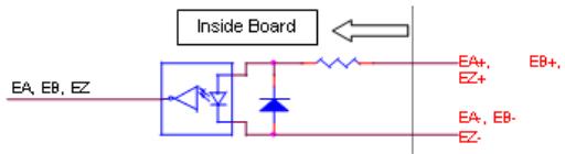
![Inside Board\nEA, EB, EZ\nEA+, EB+\nEA-, EB-\nEZ-](.sscnet-series-manual-50-1h001-1020-204/52d39b37923516119365ba6c6eeb5284dddb4452f2cb7290bf3988246de1c696.jpg)

Figure 5. Pulse input (encoder counter) circuit
Figure 4-30: Pulse Input (Encoder Counter) Circuit

Note: The voltage across each differential pair of encoder input signals (EA+, EA-), (EB+, EB-) and (EZ+, EZ-) should be at least 3.5V or higher. Therefore, the output current must be observed when connecting to the encoder feedback or motor driver feedback as not to over drive the source.

Below are examples of connecting the input signals with an external circuit. The input circuit can be connected to an encoder or motor driver, if it is equipped with: (1) a differential line driver or (2) an open collector output.

# Connection to Line Driver Output

To drive the SSCNET board encoder input, the driver output must provide at least 3.5V across the differential pairs with at least 6 mA driving capacity. The ground level of the two sides must also be tied together.

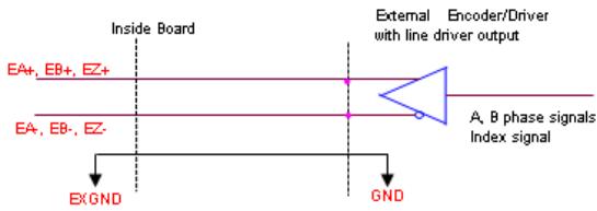
![Inside Board\nExternal Encoder/Driver\nwith line driver output\nEA+, EB+, EZ+\nEA-, EB-, EZ-\nA, B phase signals\nIndex signal\nEXGND\nGND](.sscnet-series-manual-50-1h001-1020-204/5de191708699051e9f015f682d9cfc7148e4aef29001552ae294e5bb94c6fa6c.jpg)

Figure 4-31: Line Driver Circuit

# Connection to Open Collector Output

To connect with an open collector output, an external power supply is necessary. Some motor drivers can provide the power source. The connection between the SSCNET board, encoder, and the power supply is shown in the diagram below. Note that an external current limiting resistor R is necessary to protect the SSCNET board input circuit. The following table lists the suggested resistor values according to the encoder power supply.

<table><tr><td>Encoder Power (VDD)</td><td>External Resistor R</td></tr><tr><td>+5V</td><td>0 Ω (None)</td></tr><tr><td>+12V</td><td>1.8kΩ</td></tr><tr><td>+24V</td><td>4.3kΩ</td></tr></table>

Table 4-5: Encoder Resistor

▶ +lf=6mA max.

![Based on the provided diagram, here is the accurate and concise description of the flowchart/block diagram:\n\n**Labeled Blocks and Text:**\n*   **Board** (Left side)\n*   **EA+, EB+, EZ+** (Top input signal line)\n*   **R** (Resistor)\n*   **VDD** / **GND** (Rectangular box on the top right)\n*   **External Encoder** (Text to the right of the VDD/GND box)\n*   **Power** (Text next to 'External Encoder')\n*   **Motor Encoder / Driver With Open Collector Output** (Text inside a dotted rectangular box)\n*   **EA-, EB-, EZ-** (Bottom input signal line)\n*   **A, B phase signals** (Output label)\n*   **Index signal** (Output label)\n\n**Connections:**\n*   The signal line labeled **EA+, EB+, EZ+** connects to resistor **R**.\n*   Resistor **R** connects to the left side of the box labeled **VDD** and **GND**.\n*   A line extends from the bottom of the **VDD** / **GND** box down to the base of the transistor inside the dotted box.\n*   The signal line labeled **EA-, EB-, EZ-** connects to the emitter (bottom leg with arrow) of the transistor.\n*   The transistor is enclosed within the dotted box labeled **Motor Encoder / Driver With Open Collector Output**.\n*   The collector (top leg) of the transistor connects to the output terminals labeled **A, B phase signals** and **Index signal**.](.sscnet-series-manual-50-1h001-1020-204/00c023817987a36260edb68abe381e3cd190258120808f6070e89233fa2c901d.jpg)

Figure 4-32: Open Collector Circuit

# Configuring encoder counter

Each encoder counter can be configured to receive one of the following three types of signals using the function call set\_cnt\_iptmode().

1. A/B phase (Quadrature pulse signal)
2. CW/CCW (Dual pulses signal)
3. OUT/DIR (Single Pulse signal)

# Set counter channel as position feedback of certain axis

The 3 general-purposed counters may work as position feedback source for each axis. The second parameter of the set\_cnt\_to\_axis() function defines which counter is used, the third parameter defines which axis, and the last parameter declares the resolution of the counter in units of pulses. 'Resolution' is defined as the number of pulses counted by a counter when the SSCNet motor rotates one revolution. For example:

set\_cnt\_to\_axis(0, 0, 1, 10000.0), this function will

1. Set counter '0' as position feedback source for axis '1'
2. Command the PCI-8372+ encoder to count 10000.0 pulses when motor goes one revolution.

# A/B phase

In this mode, the EA signal is $90^{\circ}$ phase leading or lagging in comparison with the EB signal. Where “lead” or “lag” is the phase difference between the two signals and is caused by the turning direction of the motor. The up/down counter counts up when the phase of the EA signal leads the phase of the EB signal.

A timing waveform is illustrated below.

![EA\nEB\nPositive Direction\nEA\nRE\nNegative Direction](.sscnet-series-manual-50-1h001-1020-204/57ebb446be3ccb6e4e3e5e9705b8f8c18cf4614faf6294ffd01ac1eca1a6b62b.jpg)

Figure 4-33: A/B Phase Timing

# CW/CCW Mode

In this mode, the pulse from EA causes the counter to count up, while EB will cause the counter to count down.

# OUT/DIR Mode

In this mode, the pulse from EB decides on whether the counter should increase or decrease, whereas EA count the number of pulses.

![EA\nEB\nPositive Direction\nNegative Direction](.sscnet-series-manual-50-1h001-1020-204/52dcb1e7a4ff99d33c5de601c8955a679835d5685bee1a9cabef4dbf78702c3f.jpg)

Figure 4-34: OUT/DIR Pulses

The index input (EZ) signal of the encoder is used as the "ZERO" index. This signal is common to most rotational motors. EZ can be used to define the absolute position of the mechanism. When a rising edge of EZ signal is received, it will clear the encoder counter value to '0'.

# Counter value read/write

To read the encoder counter value, use the get\_cnt\_value() function. The parameter ‘\*Value’ returns the counter value. To set the encoder counter value, use set\_cnt\_value(). The counter value will be set as the parameter ‘Value’.

# 4.6.2 DIO

In this section, the following functions are discussed.

```txt
get_di_status(CardID, ChNo, *Sts)
set_do_value(CardID, ChNo, Value)
```

Each PCI-8372+ board has 2-isolated digital output and 2 isolated digital input channels. Use the get\_di\_status() function to retrieve the current DI status, and set\_do\_value() to set the DO value.

# 4.6.3 DA

In this section, the following functions are discussed.

```txt
set_da_config(CardID, ChNo, Cfg)
set_da_value(CardID, ChNo, Value)
```

Each SSCNET board has 2 analog voltage output channels and can be independently configured using the set\_da\_config() function to set the DA to either be a direct DA output or for a velocity profile output. The default setting is DA direct output.

By using direct DA output, users can control the DA value using the set\_da\_value() function. While using velocity profile output will cause the DA output value to be proportional to the current command velocity. E.g. when a motor is rotating at 3000 rpm, the DA output is 10V and the DA output would be -10V if the rotating speed is -3000 rpm.

![| Axis rotating speed (rpm) | DA output Voltage (Volt) |\n| :--- | :--- |\n| -3000 | 10 |\n| 3000 | 10 |](.sscnet-series-manual-50-1h001-1020-204/49a795c32bb670376e2f07a23b4c346764566ad716a1e347a977cc6bf1613877.jpg)

Figure 4-35: DA Output

# 4.6.4 AD

In this section, the following functions are discussed.

```txt
set_ad_function(CardID, Enable, AD_gain, AD_Last, AD2_src)
get_da_value(CardID, ChNo, *Value)
```

There are two analog input channels on the cPCI-8212H. It is used for sensing anlog output device ranged from -10V to +10V. Users can choose the gain by 1, 2, or 4. It means that the input voltage range could be +/-10V, +/-5V and +/- 2.5V for optimizing input resolution. There is an internal analog input channel which is for double checking. It is called AD2. The source of this channel could be chosen from internal +5V, ground, DA0, or DA1. It is very useful in debugging.

# 4.6.5 Analog channel auto calibration

In this section, the following functions are discussed.

```txt
tune_ref_5V(CardID, Value)
save_auto_k_value(CardID, Channel, Value)
get_auto_k_value(CardID, Channel, *Value)
tune_ad_offset_gain(CardID, Step, Value)
tune_da_offset(CardID, Step, Value)
reload_auto_k_setting(CardID)
```

In the past, the calibration of analog I/O needs many VRs to finished it. Now, SSCNET board has built-in the electric VRs in PLD. Users needn't use screw driver to tune the value of offset or gain anymore. They need only set the values like tuning VR via those functions we provided. Users needn't to tune these value because we have done this when this board is produced. The procedure of tuning these analog channels are as following:

1. Tune the on board +5V generator to exactly +5.0000V by measuring it from JP1 connector on daughter board. PCI-8372+/8366+ don't have this feature.
2. Execute tune\_ad\_offset\_gain() by Step=1, Value=128.
PCI-8372+/8366+ don't have this feature.
3. Execute tune\_ad\_offset\_gain() by Step=3, Value=128.
PCI-8372+/8366+ don't have this feature.
4. Calibrate AD offset using tune\_ad\_offset\_gain() for Step=0. Check AD2's value as 0.0. PCI-8372+/8366+ does not have this feature.
5. Calibrate AD offset using tune\_ad\_offset\_gain() for Step=1. Check AD2's value as 0.0. PCI-8372+/8366+ does not have this feature.
6. Calibrate AD gain using tune\_ad\_offset\_gain() for Step=2. Check AD2's value as 5.0. PCI-8372+/8366+ does not have this feature.
7. Execute tune\_da\_offset() by Step=1, Value=128.
8. Execute tune\_da\_offset() by Step=3, Value=128.
9. Calibrate DA offset using tune\_da\_offset() for Step=0. Check AD2's value as 0.0.
10. Calibrate DA offset using tune\_da\_offset() for Step=1. Check AD2's value as 0.0.
11. Calibrate DA offset using tune\_da\_offset() for Step=2. Check AD2's value as 0.0.
12. Calibrate DA offset using tune\_da\_offset() for Step=3. Check AD2's value as 0.0.
13. Execute save\_auto\_k\_value() and the tuning value above will be saved in EEPROM on the board. These values will be restored by reload\_auto\_k\_value() when board is initialized.

# 4.7 Driver Management

# 4.7.1 Driver parameter

In this section, the following functions are discussed.

```c
get_servo_para(Axis, ParaNo,*Value)
set_servo_para(Axis, ParaNo, Value)
get_servo_para_all(Axis, *Value)
set_servo_para_all(Axis, *Value)
save_servo_para(I16 Axis)
set_servo_para_default(I16 Axis)
```

With the SSCNET board, servo parameters read/write becomes very easy using function calls listed above.

To read a current parameter setting, user can call get\_servo\_para() or get\_servo\_para\_all(). get\_servo\_para() retrieves certain parameter values, while get\_servo\_para\_all() will retrieve all parameter settings.

To set a new value for the servo parameters, user can call set\_servo\_para() or set\_servo\_para\_all(). set\_servo\_para() will set new values for specified parameters only, while set\_servo\_para\_all() will set all parameters' value.

After a servo parameter tuning process, user may use save\_servo\_para() to store current parameter setting. These values are stored in a Flash ROM of the SSCNET board.

Whenever the user wants to restore default parameter setting, the function set\_servo\_para\_default() can be used. This will reset all parameters to the factory setting.

The following table is a simplified list of parameters. For more information, refer to the “MR-J2SB Instruction Manual”.

<table><tr><td>Symbol</td><td>Name</td><td>MR-J2SB Instruction Manual Parameter</td><td>Unit</td><td>Setting Range</td></tr><tr><td>*AMS</td><td>Amp setting</td><td>Pr.01</td><td></td><td>0000H~0001H</td></tr><tr><td>*REG</td><td>Regenerative resistor</td><td>Pr.02</td><td></td><td>0000H~0011H</td></tr><tr><td>*MTY</td><td>For manufacturer&#x27;s settings</td><td>Pr.03</td><td></td><td>0080H</td></tr></table>

Table 4-6: MR-J2SB Parameters

<table><tr><td>Symbol</td><td>Name</td><td>MR-J2SB Instruction Manual Parameter</td><td>Unit</td><td>Setting Range</td></tr><tr><td>*MCA</td><td>For manufacturer&#x27;s settings</td><td>Pr.04</td><td></td><td>0000H</td></tr><tr><td>*MTR</td><td>For manufacturer&#x27;s settings</td><td>Pr.05</td><td></td><td>1</td></tr><tr><td>*FBP</td><td>Feedback pulse number</td><td>Pr.06</td><td></td><td>0,1,6,7,225</td></tr><tr><td>*POL</td><td>Direction of motor rotation</td><td>Pr.07</td><td></td><td>0,1</td></tr><tr><td>ATU</td><td>Auto-tuning</td><td>Pr.08</td><td></td><td>0000H~0004H</td></tr><tr><td>RSP</td><td>Servo response setting</td><td>Pr.09</td><td></td><td>0001H~000FH</td></tr><tr><td>TLP</td><td>Forward rotation torque lim-its</td><td>Pr.10</td><td>%</td><td>0~Maximum torque</td></tr><tr><td>TLN</td><td>Reverse rotation torque limits</td><td>Pr.11</td><td>%</td><td>0~Maximum torque</td></tr><tr><td>DG2</td><td>Moment of inertia ratio of load</td><td>Pr.12</td><td>0.1</td><td>0~3000</td></tr><tr><td>PG1</td><td>Position control gain 1</td><td>Pr.13</td><td>rad/sec</td><td>4~2000</td></tr><tr><td>VG1</td><td>Speed control gain 1</td><td>Pr.14</td><td>rad/sec</td><td>20~8000</td></tr><tr><td>PG2</td><td>Position control gain 2</td><td>Pr.15</td><td>rad/sec</td><td>1~1000</td></tr><tr><td>VG2</td><td>Speed control gain 2</td><td>Pr.16</td><td>rad/sec</td><td>20~20000</td></tr><tr><td>VIC</td><td>Speed integration compen-sation</td><td>Pr.17</td><td>msec</td><td>1~1000</td></tr><tr><td>NCH</td><td>Mechanical resonance con-trol filter</td><td>Pr.18</td><td></td><td>0~031FH</td></tr><tr><td>FFC</td><td>Feed forward gain</td><td>Pr.19</td><td>%</td><td>0~100</td></tr><tr><td>INP</td><td>In position range</td><td>Pr.20</td><td>pulse</td><td>0~50000</td></tr><tr><td>MBR</td><td>Electromagnetic brake sequence output</td><td>Pr.21</td><td>msec</td><td>0~1000</td></tr><tr><td>MOD</td><td>Monitor output mode</td><td>Pr.22</td><td></td><td>0000H~0B0BH</td></tr><tr><td>OP1</td><td>Optional function 1</td><td>Pr.23</td><td></td><td>0000H~0001H</td></tr><tr><td>OP2</td><td>Optional function 2</td><td>Pr.24</td><td></td><td>0000H~0110H</td></tr><tr><td>LPF</td><td>Low pass filter</td><td>Pr.25</td><td></td><td>0000H~1210H</td></tr><tr><td>OP4</td><td>For manufacturer&#x27;s settings</td><td>Pr.26</td><td></td><td>0000H</td></tr><tr><td>MO1</td><td>Monitor output 1 offset</td><td>Pr.27</td><td>mv</td><td>-999~999</td></tr><tr><td>MO2</td><td>Monitor output 2 offset</td><td>Pr.28</td><td>Mv</td><td>-999~999</td></tr></table>

Table 4-6: MR-J2SB Parameters

<table><tr><td>Symbol</td><td>Name</td><td>MR-J2SB Instruction Manual Parameter</td><td>Unit</td><td>Setting Range</td></tr><tr><td>MOA</td><td>For manufacturer&#x27;s settings</td><td>Pr.29</td><td></td><td>0001H</td></tr><tr><td>ZSP</td><td>Zero speed</td><td>Pr.30</td><td>rpm</td><td>0~10000</td></tr><tr><td>ERZ</td><td>Error excess alarm level</td><td>Pr.31</td><td>kpulse</td><td>1~1000</td></tr><tr><td>OP5</td><td>Option function 5</td><td>Pr.32</td><td></td><td>0000H~0002H</td></tr><tr><td>OP6</td><td>For manufacturer&#x27;s settings</td><td>Pr.33</td><td></td><td>0000H~0113H</td></tr><tr><td>VPI</td><td>PI-PID change position droop</td><td>Pr.34</td><td></td><td>0~50000</td></tr><tr><td>TTT</td><td>For manufacturer&#x27;s settings</td><td>Pr.35</td><td></td><td>0000H</td></tr><tr><td>VDC</td><td>Speed integration compensation</td><td>Pr.36</td><td></td><td>0~1000</td></tr><tr><td>OP7</td><td>For manufacturer&#x27;s settings</td><td>Pr.37</td><td></td><td>0010H</td></tr><tr><td>ENR</td><td>Encoder output pulse</td><td>Pr.38</td><td></td><td>0~32768</td></tr><tr><td></td><td>For manufacturer&#x27;s settings</td><td>Pr.39</td><td></td><td>0000H</td></tr><tr><td>*BLK</td><td>Parameter block</td><td>Pr.40</td><td></td><td>0000H~000EH</td></tr></table>

Table 4-6: MR-J2SB Parameters

# 4.7.2 Data monitoring

In this section, the following functions are discussed.

```txt
set_monitor_channel(Axis, Channel_0, Channel_1, Channel_2, Channel_3)
set_monitor_config(Axis, Trigger_Select, Trigger_Level, SamplePeriod, PreTriggerSampleNo, SampleNumber)
get_instant_monitor_data(Axis,*Data_0,*Data_1,*Data_2, *Data_3)
start_monitor(Axis)
check_monitor_ready(Axis, *status)
get_monitor_data(Axis, *Data)
```

The firmware in the SSCNET board gives each axis 4 monitoring channels. Users can use these monitoring channels to monitor a variety of I/O data, such as Speed feedback, INP (in position)... etc.

To be able to use the monitoring function, users must understand the configuring and operating procedures.

# Configuring procedures:

Configuring procedure is necessary before a monitor function can be started. There are two main instructions during configuration:

# 1. set\_monitor\_channel

This function is used to set the monitoring target. This function must be executed before monitoring can started.

The first parameter ‘Axis’ specifies the axis. The remaining four parameters are used for the monitoring targets. The relationship between set values and monitoring targets are list below.

<table><tr><td>Value</td><td>Description</td><td>Unit</td></tr><tr><td>FF</td><td>Not Used</td><td></td></tr><tr><td>00</td><td>Feedback pulse accumulation</td><td>Pulse</td></tr><tr><td>01</td><td>(Reserved)</td><td></td></tr><tr><td>02</td><td>Motor revolution speed</td><td>0.1rpm</td></tr><tr><td>03</td><td>(Reserved)</td><td></td></tr><tr><td>04</td><td>Accumulated pulse</td><td>Pulse</td></tr><tr><td>05</td><td>(Reserved)</td><td></td></tr><tr><td>06</td><td>Regenerative load factor</td><td>%</td></tr><tr><td>07</td><td>Execution load factor</td><td>%</td></tr><tr><td>08</td><td>Peak load factor</td><td>%</td></tr><tr><td>09</td><td>Bus voltage</td><td></td></tr><tr><td>0A</td><td>Load inertia ratio</td><td></td></tr><tr><td>0B</td><td>ABS counter</td><td>Rev</td></tr><tr><td>0C</td><td>Position within one revolution</td><td>Pulse</td></tr><tr><td>0D</td><td>(Reserved)</td><td></td></tr><tr><td>0E</td><td>F/B present value</td><td>Pulse</td></tr><tr><td>0F</td><td>(Reserved)</td><td></td></tr><tr><td>10</td><td>Position droop</td><td>Pulse</td></tr><tr><td>11</td><td>(Reserved)</td><td></td></tr><tr><td>12</td><td>Speed command</td><td>0.1rpm</td></tr><tr><td>13</td><td>(Reserved)</td><td>0.1rpm</td></tr><tr><td>14</td><td>Speed feedback</td><td>0.1rpm</td></tr><tr><td>15</td><td>(Reserved)</td><td>0.1rpm</td></tr><tr><td>16</td><td>Current command</td><td>0.1%</td></tr><tr><td>17</td><td>Current feedback</td><td>0.1%</td></tr><tr><td>18</td><td>ZCT (Bottom)</td><td>Pulse</td></tr><tr><td>19</td><td>(Reserved)</td><td></td></tr><tr><td>1A</td><td>Present revolution counts</td><td>Rev</td></tr></table>

Table 4-7: Monitoring Targets

<table><tr><td>Value</td><td>Description</td><td>Unit</td></tr><tr><td>1B</td><td>Origin revolution counts</td><td>Rev</td></tr><tr><td>1C</td><td>Origin position within one revolution</td><td>Pulse</td></tr><tr><td>1D</td><td>(Reserved)</td><td></td></tr><tr><td>1E</td><td>(Reserved)</td><td></td></tr><tr><td>1F</td><td>(Reserved)</td><td></td></tr><tr><td>20</td><td>Alarm status AL-1</td><td></td></tr><tr><td>21</td><td>Alarm status AL-2</td><td></td></tr><tr><td>22</td><td>Alarm status AL-3</td><td></td></tr><tr><td>23</td><td>Alarm status AL-4</td><td></td></tr><tr><td>24</td><td>Alarm status AL-5</td><td></td></tr><tr><td>25</td><td>Alarm status AL-6</td><td></td></tr><tr><td>26</td><td>Alarm status AL-7</td><td></td></tr><tr><td>27</td><td>Alarm status AL-8</td><td></td></tr><tr><td>28</td><td>Alarm status AL-9</td><td></td></tr><tr><td>29</td><td>Alarm status AL-E</td><td></td></tr><tr><td>2A</td><td>(Reserved)</td><td></td></tr><tr><td>2B</td><td>(Reserved)</td><td></td></tr><tr><td>2C</td><td>(Reserved)</td><td></td></tr><tr><td>2D</td><td>(Reserved)</td><td></td></tr><tr><td>2E</td><td>(Reserved)</td><td></td></tr><tr><td>2F</td><td>(Reserved)</td><td></td></tr><tr><td>30</td><td>Alarm history #1,#2</td><td></td></tr><tr><td>31</td><td>Alarm history #3,#4</td><td></td></tr><tr><td>32</td><td>Alarm history #5,#6</td><td></td></tr><tr><td>33</td><td>Alarm history #7,#8</td><td></td></tr><tr><td>34</td><td>Alarm history #9,#10</td><td></td></tr><tr><td>35</td><td>(Reserved)</td><td></td></tr><tr><td>36</td><td>(Reserved)</td><td></td></tr><tr><td>37</td><td>(Reserved)</td><td></td></tr><tr><td>38</td><td>Parameter error NO.Pr01 to Pr16</td><td></td></tr><tr><td>39</td><td>Parameter error NO.Pr17 to Pr32</td><td></td></tr><tr><td>3A</td><td>Parameter error NO.Pr33 to Pr40</td><td></td></tr></table>

Table 4-7: Monitoring Targets

<table><tr><td>Value</td><td>Description</td><td>Unit</td></tr><tr><td>3B</td><td>(Reserved)</td><td></td></tr><tr><td>3C</td><td>(Reserved)</td><td></td></tr><tr><td>3D</td><td>(Reserved)</td><td></td></tr><tr><td>3E</td><td>(Reserved)</td><td></td></tr><tr><td>3F</td><td>(Reserved)</td><td></td></tr><tr><td>A5</td><td>INP (in position)</td><td>Active: 1, Inactive: 0</td></tr><tr><td>B0</td><td>Velocity Command</td><td>Pulse/sec</td></tr><tr><td>B2</td><td>DA1 Value</td><td></td></tr><tr><td>B3</td><td>DA2 Value</td><td></td></tr><tr><td>B4</td><td>Speed Feedback</td><td></td></tr><tr><td>B6</td><td>External Encoder Feedback</td><td></td></tr><tr><td>B8</td><td>Command Pulse</td><td></td></tr></table>

Table 4-7: Monitoring Targets

# 2. set\_monitor\_config

This function is used to set the monitoring configuration, such as sampling period, trigger condition...etc. This function must be executed before monitoring can start.

The first parameter ‘Axis’ specifies which axis. Other parameters are listed below.

<table><tr><td>Parameter Name</td><td>Description</td></tr><tr><td rowspan="11">Trigger_Select</td><td>This variable is used to define the trigger source.</td></tr><tr><td>Trigger_Select:</td></tr><tr><td>Value = 0: No trigger</td></tr><tr><td>Value = 1: CH0 as trigger source, going high</td></tr><tr><td>Value = 2: CH1 as trigger source, going high</td></tr><tr><td>Value = 3: CH2 as trigger source, going high</td></tr><tr><td>Value = 4: CH3 as trigger source, going high</td></tr><tr><td>Value = -1: CH0 as trigger source, going low</td></tr><tr><td>Value = -2: CH1 as trigger source, going low</td></tr><tr><td>Value = -3: CH2 as trigger source, going low</td></tr><tr><td>Value = -4: CH3 as trigger source, going low</td></tr><tr><td>TriggerLevel</td><td>Define the trigger level</td></tr><tr><td rowspan="5">SamplePeriod</td><td>This variable is used to define the sample period.</td></tr><tr><td>Value = 1: 0.888 ms</td></tr><tr><td>Value = 2: 2 * 0.888 ms</td></tr><tr><td>Value = 3: 3 * 0.888 ms</td></tr><tr><td>Value = 4: 4 * 0.888 ms</td></tr><tr><td rowspan="2">PreTriggerSampleNo</td><td>Define the Number of samples before Trigger</td></tr><tr><td>Value = 1 ~ 1023</td></tr><tr><td rowspan="2">SampleNumber</td><td>Define the Total Number of samples</td></tr><tr><td>Value = 1 ~ 1023</td></tr></table>

Table 4-8: Axis Parameters

# Operating procedures:

There are 2 operation modes, real time data reading and normal monitoring.

# 1. get\_instant\_monitor\_data

After the monitoring channels have been set by set\_monitor\_channel(), the get\_instant\_monitor\_data() function can be used to retrieve monitoring data.

The first parameter ‘Axis’ specifies which axis. The remaining four parameters are used to retrieve monitoring data from the monitoring channels.

This function returns a value immediately and carries out real time monitoring of specified monitoring targets.

# 2. Normal monitoring

Normal monitoring is data sampling with the help of the on-board DSP. The DSP take charge of storing all sampled data according to configuration set by set\_monitor\_config(). The following steps are necessary to operate in normal monitoring.

Step 0: Set monitor channel and configuration using function call: set\_monitor\_channel(), set\_monitor\_config()

Step 1: Start normal monitoring using the function call: start\_monitor(). This will start the DSP.

Step 2: Check if the monitoring has completed by calling the function: check\_monitor\_ready(). The parameter 'status' returns a value, if the monitoring process has completed.

Step 3: If monitoring has completed, then call get\_monitor\_data() to retrieve the monitored data.

The size of the 'data' array of the function get\_monitor\_data(), which is used to read the monitored data must be 4 times the value of 'PreTriggerSampleNo' in set\_monitor\_config() and when the function get\_monitor\_data() returns a value, the 'data' is stored in the following format.

Data array

<table><tr><td>Channel 0, data 0</td><td>0</td></tr><tr><td>Channel 0, data 1</td><td>1</td></tr><tr><td>Channel 0, data 2</td><td>2</td></tr><tr><td>......</td><td>:</td></tr><tr><td>......</td><td>PreTriggerSampleNo - 1</td></tr><tr><td>Channel 1, data 1</td><td>PreTriggerSampleNo + 0</td></tr><tr><td>Channel 1, data 2</td><td>PreTriggerSampleNo + 1</td></tr><tr><td>......</td><td>:</td></tr><tr><td>......</td><td>2*PreTriggerSampleNo - 1</td></tr><tr><td>Channel 2, data 0</td><td>2*PreTriggerSampleNo + 0</td></tr><tr><td>Channel 2, data 1</td><td>2*PreTriggerSampleNo + 1</td></tr><tr><td>Channel 2, data 2</td><td>2*PreTriggerSampleNo + 2</td></tr><tr><td>......</td><td>:</td></tr><tr><td>......</td><td>3*PreTriggerSampleNo - 1</td></tr><tr><td>Channel 3, data 0</td><td>3*PreTriggerSampleNo + 0</td></tr><tr><td>Channel 3, data 1</td><td>3*PreTriggerSampleNo + 1</td></tr><tr><td>Channel 3, data 2</td><td>2*PreTriggerSampleNo + 2</td></tr><tr><td>......</td><td>:</td></tr><tr><td>......</td><td>4*PreTriggerSampleNo - 1</td></tr></table>

Offset
Table 4-9: Data Array Offset

# 4.7.3 Servo Information

In this section, the following function is discussed.

get\_servo\_info(Axis, \*ServoInfo)

This function is used to retrieve the servo driver's status information. The parameter ‘\*Servolinfo’ carries the information about servo driver's status in individual bit's:

<table><tr><td>Bit 0</td><td>In Ready-ON</td></tr><tr><td>Bit 1</td><td>In Servo-ON</td></tr><tr><td>Bit 2</td><td>In course of in-Position</td></tr></table>

Table 4-10: Servo Bit Information

<table><tr><td>Bit 3</td><td>In course of zero speed</td></tr><tr><td>Bit 4</td><td>Pass through Z phase of servo motor</td></tr><tr><td>Bit 5</td><td>In Torque limit</td></tr><tr><td>Bit 6</td><td>In Alarm</td></tr><tr><td>Bit 7</td><td>In warning</td></tr><tr><td>Bit 8</td><td>Reserve</td></tr><tr><td>Bit 9</td><td>Reserve</td></tr><tr><td>Bit 10 ~ 14</td><td>Reserved</td></tr><tr><td>Bit 15</td><td>In course of Speed limit</td></tr><tr><td>Bit 16 ~ 31</td><td>Reserved</td></tr></table>

Table 4-10: Servo Bit Information

# 4.7.4 Servo On

In this section, the following function is discussed.

```python
set_servo_on(Axis, ON_OFF)
```

After this function is execute with 'ON\_OFF' = 1, the servo driver of specified axis starts to control its servomotor. Motion functions can now be applied to the axis.

In most cases, Servo driver should be at servo ON status, except that, "Before set\_position() function, the servo driver must be at Servo OFF status."

# 4.7.5 Driver information

In this section, the following functions are discussed.

```txt
understand_driver(Axis, *Class_Code)
understand_motor(Axis, *MotorType, *Capacity,
*RateRPM, *RateCurrent, *MaxRPM, *MaxTorq,
*PPR, *ENCInfo, *OptionalInfor)
```

When booting, the SSCNET board will gather some static information about the servo driver and servomotor. This information is kept by the SSCNET board and users can retrieve the info using the following two functions.

To read the servo driver's static info, use understand\_driver()
To read servo motor's static info, use understand\_motor()

# 4.7.6 Servo Alarm

In this section, the following functions are discussed.

```python
get_alarm_no(Axis, *AlarmNo)
alarm_reset(Axis)
```

When a fault occurs, the servo driver will stop the motor and report an alarm number on the LED display of the servo driver. The SSCNET board will also be acknowledged because the servo driver also reports the alarm condition through SSCNet communication. If this is the case, users can exam the fault condition by:

1. Examining the return code from the function call.
2. Set an IRQ. Allow a IRQ to be generated, if an alarm occurs. Refer to section 4.9.

After noticing the occurrence of the alarm, users can use get\_alarm\_no() to retrieve the alarm code, which is displayed on the LED of the servo driver. After removing the alarm condition, users can use the alarm\_reset() function to recover the driver from the alarm state.

# 4.8 Control Gain Tuning

In this section, the following functions are discussed.

```txt
set_auto_tune(Axis, Mode, RSP, GD2)
get_auto_tune(Axis, *Mode, *RSP, *GD2)
set_control_gain(Axis, PG1, VG1, VIC, PG2, VG2, FFC)
get_control_gain(Axis, *PG1, *VG1, *VIC, *PG2, *VG2, *FFC)
set_notch_filter(Axis, Mode, NotchFrequency, NotchDepth)
get_notch_filter(Axis, *Mode, *NotchFrequency, *NotchDepth)
set_LP_filter(Axis, ON_OFF)
```

get\_LP\_filter(Axis, \*ON\_OFF)

# 4.8.1 Control Gains

The first 4 functions are used to set/read the gain controls of the servomotor control system. There are 6 control gains, and they are PG1, VG1, VIC, PG2, VG2, and FFC. The following are some simple description of the control gains, for more information refers to the “Instruction Manual” of the MR-J2S-B servo driver.

# PG1: Position loop gain 1

Increase this value to improve tractability in response to the position command.

# VG1: Velocity loop gain 1

Normally this gain value does not need to be changed. A higher set value increases the response level but is likely to generate vibration and/or noise.

# VIC: Velocity integral compensation

Used to set the integral time constant of a speed loop. A higher set value increases the response level but is likely to generate vibration and/or noise.

# PG2: Position loop gain 2

This gain is used to increase the response due to level load disturbance. A higher set value increases the response level but is likely to generate vibration and/or noise.

# VG2: Velocity loop gain 2

Set this gain when vibration occurs to machines with low rigidity or with large backlash. A higher set value increases the response level but is likely to generate vibration and/or noise.

# FFC: Feed foreword gain

Used to set the velocity feed foreword gain. When it is set to 100%, drop pulses will be almost zero at constant-speed operation. Note that higher set values will increase response but will enlarge the overshoot during sudden acceleration/deceleration.

# Auto-Tuning mode

The MR-J2S-B servo driver has as read-time auto tuning function, which can automatically estimate the machines characteristic and set the optimum control gain values in real time.

There are two Auto-Tuning modes:

Auto-Tuning mode 1:

In this mode, the load inertia moment of a machine is estimated, and all control gains are set automatically, creating a machine response frequency that matches the user's requirements (RSP). The servo driver is factory-set to this mode.

Under this mode, set\_control\_gain() does not work and will return errors.

Auto-Tuning mode 2:

Under this mode, the user must specify the load inertia moment for the machine (GD2) with all other control gains set automatically, creating a machine response frequency that matches the user's requirements (RSP).

Under this mode, set\_control\_gain() does not work and will return errors.

# Manual setting mode

If the user is not satisfied with the adjustment of auto-tuning, he/she can make manual adjustments.

Manual mode 1:

Under this mode, the user can specify the following control gains including GD2, PG1, VG2, and VIC, while PG2 VG1 and FFC are set automatically.

Under this mode, set\_control\_gain() can be used to set PG1, VG2, and VIC. Setting for PG2, VG1 and FFC is automatically ignored.

Manual mode 2:

Under this mode, the user can specify all control gains. The function call set\_control\_gain() can be used to set PG1, VG2, VIC, PG2, VG2 and FFC.

The function call set\_auto\_tune() is used to select the auto-tuning or manual tuning mode with the parameter 'Mode' specifying the operation mode. If Auto-tuning mode is selected, 'RSP' specifies the user's machine response frequency requirements, while in manual mode it's not applicable. 'GD2' specifies the load inertia moment of a machine.

The function call get\_auto\_tune() can be used to read settings from the servo driver.
The function call set\_control\_gain() is used to set the control gains when manual mode operation is selected.
The function call get\_auto\_tune() can be used to read settings from the servo driver.
▶ The following table is a list of selectable gains under different operation modes:

<table><tr><td>‘Mode’ Value</td><td>Description</td><td>RSP</td><td>GD2</td><td>PG1</td><td>VG1</td><td>VIC</td><td>PG2</td><td>VG2</td><td>FFC</td></tr><tr><td>1</td><td>Auto-Tuning mode 1</td><td>M</td><td>A</td><td>A</td><td>A</td><td>A</td><td>A</td><td>A</td><td>A</td></tr><tr><td>2</td><td>Manual mode 2</td><td>--</td><td>M</td><td>M</td><td>M</td><td>M</td><td>M</td><td>M</td><td>M</td></tr><tr><td>3</td><td>Auto-Tuning mode 2</td><td>M</td><td>M</td><td>A</td><td>A</td><td>A</td><td>A</td><td>A</td><td>A</td></tr><tr><td>4</td><td>Manual mode 1</td><td>--</td><td>M</td><td>M</td><td>A</td><td>M</td><td>A</td><td>M</td><td>A</td></tr><tr><td>0*</td><td>Interpolation mode</td><td>--</td><td>A</td><td>M</td><td>M</td><td>A</td><td>A</td><td>A</td><td>A</td></tr></table>

Table 4-11: Selectable Gains

▶ A: automatically set
▶ M: manually specify
▶ --: Not used
▶ \* Interpolation mode is normally not used.

# 4.8.2 Mechanical resonance suppression filter

The functions set\_notch\_filter() and get\_notch\_filter() are related to the mechanical resonance suppression filter function.

If a mechanical system has a natural resonance point, increasing the servo system response may cause the mechanical system to produce resonance (vibration) at its resonance frequency. Using the notch filter and adaptive vibration suppression control functions can suppress the resonance of the mechanical system.

# Notch filter

The notch filter is a filter function, which decreases the gain of the specific frequency (notch frequency) and gain decreasing depth.

![| Frequency | Mechanical system response | Notch Depth |\n| --------- | -------------------------- | ----------- |\n| 0         | High                       | Low         |\n| 2.5       | Medium                     | Low         |\n| 3.0       | Low                        | Very Low    |\n| 4.0       | Very Low                   | Low         |\n| 5.0       | Very Low                   | Very Low    |](.sscnet-series-manual-50-1h001-1020-204/6f989830b4b62bfd9037ebc78d67536f7366f880ed6726a6b739a0ba8a3a292d.jpg)

Figure 4-36: Notch Filter

Note: The machine resonance suppression filter is a delay factor for the servo system. Hence, vibration may increase if you set a wrong resonance frequency or a too deep notch.

If the resonance frequency of the machine is unknown, decrease the notch frequency from a higher to lower order. The optimum notch frequency is set at the point where vibration is minimal.

The notch frequency is set with the parameter 'NotchFrequency'. The setting values and corresponding notch frequency are listed in the table below.

<table><tr><td>Setting</td><td>Frequency</td><td>Setting</td><td>Frequency</td><td>Setting</td><td>Frequency</td><td>Setting</td><td>Frequency</td></tr><tr><td>0</td><td>Invalid</td><td>8</td><td>562.5</td><td>16</td><td>281.3</td><td>24</td><td>187.5</td></tr><tr><td>1</td><td>4500</td><td>9</td><td>500</td><td>17</td><td>264.7</td><td>25</td><td>180</td></tr><tr><td>2</td><td>2250</td><td>10</td><td>450</td><td>18</td><td>250</td><td>26</td><td>173.1</td></tr><tr><td>3</td><td>1500</td><td>11</td><td>409.1</td><td>19</td><td>236.8</td><td>27</td><td>166.7</td></tr><tr><td>4</td><td>1125</td><td>12</td><td>375</td><td>20</td><td>225</td><td>28</td><td>160.1</td></tr><tr><td>5</td><td>900</td><td>13</td><td>346.2</td><td>21</td><td>214.3</td><td>29</td><td>155.2</td></tr><tr><td>6</td><td>750</td><td>14</td><td>321.4</td><td>22</td><td>204.5</td><td>30</td><td>150</td></tr><tr><td>7</td><td>642.9</td><td>15</td><td>300</td><td>23</td><td>195.7</td><td>31</td><td>145.2</td></tr></table>

Table 4-12: Notch Frequency Settings

A deeper notch provides better resonance suppression but increases the phase delay and may increase vibration.

The notch frequency can be set with the parameter 'NotchDepth'. The setting values and corresponding notch gain are listed in the table below.

<table><tr><td>Setting</td><td>Depth (Gain)</td></tr><tr><td>0</td><td>-40db</td></tr><tr><td>1</td><td>-14db</td></tr><tr><td>2</td><td>-8db</td></tr><tr><td>3</td><td>-4db</td></tr></table>

Table 4-13: Notch Gain Settings

# Adaptive vibration suppression control

Adaptive vibration suppression control is a function in which the servo driver detects machine's resonance and set a adaptive filter (also a notch filter) automatically to suppress mechanical system vibration.

Note: This adaptive filter has nothing to do with previous Notch filter setting.

Since the adaptive filter characteristics (notch frequency and depth) are set automatically, user need not be conscious of the resonance frequency of a mechanical system. Also, while adaptive vibration suppression control is valid, the servo driver always detects machine resonance, and if the resonance frequency changes, it changes the filter characteristics in response to that frequency.

The Adaptive vibration suppression control function can be set with the parameter ‘Mode’. The setting value and suppression control function are listed in the table below.

<table><tr><td>Setting</td><td>Control Selection</td></tr><tr><td>0</td><td>Invalid - The adaptive vibration suppression control is not used.</td></tr></table>

Table 4-14: Suppression Control Settings

<table><tr><td>Setting</td><td>Control Selection</td></tr><tr><td>1</td><td>Valid_0 - The adaptive vibration suppression control is enabled with normal sensitivity of detecting machine resonance.</td></tr><tr><td>2</td><td>Valid_1 - The adaptive vibration suppression control is enabled with large sensitivity of detecting machine resonance.</td></tr><tr><td>3</td><td>Hold - filter characteristic generated so far is held, and detection of machine resonance is stopped.</td></tr></table>

Table 4-14: Suppression Control Settings

Note: 1. The mode setting does not affect the notch filters functionality set by 'NotchFrequency' and 'NotchDepth'
2. Adaptive vibration control is factory-set to be invalid.
3. Adaptive vibration control is useful only when machine resonance is between 150 \~ 500 Hz. It has no effect on the resonance frequency outside this range.
4. Under operating conditions in which sudden disturbance is imposed during operation, the detection of the resonance frequency may malfunction temporarily, causing machine vibration. In such a case, set the adaptive vibration suppression control mode to be 3 (Hold) to fix the characteristics of the adaptive vibration suppression control filter.

# 4.8.3 Low pass filter

The functions set\_LP\_filter() and get\_LP\_filter() are related to low pass filter functions.

When a ball-screw or the like is used, resonance of high frequency may occur as the response of the servo system is increased. To prevent this, the low-pass filer is factory-set to be valid with a torque command. The filtering frequency of this low pass filter is automatically adjusted to the value according to the expression below:

VG2 setting\* 10

Filter Frequency (Hz) = \_\_\_\_

$2*\pi*(1+GD2\text{ setting }0.1)$

The low pass filter can be enabled or disabled using the parameter 'ON\_OFF'.

▶ 'ON\_OFF' = 0, Disabled
▶ 'ON\_OFF' = 1, Enabled

Note: In a mechanical system where rigidity is extremely high and resonance's difficult to occur, setting the low pass filter to be 'Disabled' may increase the servo system response to shorten the settling time.

# 4.9 Interrupt control

In this section, the following functions are discussed.

```txt
int_control(CardID, Flag)
set_int_factor(CardID, Source, IntFactor)
get_int_status(CardID, Source, *IntStatus)
set_int_event(CardID, *HEvent)
link_interrupt(CardID, *callbackAddr)
```

The SSCNET board can generate an interrupt for certain conditions. Refer to the figure below:

![The flowchart depicts a system architecture with four main labeled blocks and their connections:\n\n**Blocks:**\n*   **SSCNET board** (Bottom)\n*   **DLL & Driver** (Middle)\n*   **User AP** (Top container)\n    *   Inside the **User AP** box, there are two sub-blocks:\n        *   **Call routine back** (Left)\n        *   **Thread waiting for event** (Right)\n\n**Connections:**\n*   An arrow points upward from **SSCNET board** to **DLL & Driver**.\n*   Two arrows originate from **DLL & Driver** and point upward into the **User AP** container.\n    *   A dotted line connects the two arrows near their base.\n    *   One arrow points to the **Call routine back** block.\n    *   The other arrow points to the **Thread waiting for event** block.](.sscnet-series-manual-50-1h001-1020-204/3abc4a31648a4e08b4966f6f13bcc0fb6ce8fdc8742dd16a7b5089741e103178.jpg)

Figure 4-37: Interrupt Control

Users can either set a call back routine that will be executed when an interrupt occurs, or create a thread to wait for an event that will be triggered when an interrupt occurs.

To enable or disable the interrupt generated from the SSCNET board, use the int\_control() function. It acts as an ON\_OFF switch. Once disabled, the SSCNET board will cease to generate any interrupt signals to the host system.

In addition to int\_control(), users need to define the conditions under which an interrupt signal should occurs by using the set\_int\_factor() function in order to successfully introduce an interrupt signal to the host system. The SSCNET board has 3 possible sources of interrupts; it includes the motion axes, general purpose I/O, and the DSP (or system). The second parameter 'Source' of set\_int\_factor() is use to specify the source with 'IntFactor' specifying the interrupt conditions for this specified source.

Refer to the tables below.

“Source” = 0 - 11, for Axis 0 - Axis 11 respectively.

<table><tr><td>Bit of ‘IntFactor’</td><td>Name</td><td>Description</td></tr><tr><td>0</td><td>PEL</td><td>Positive Limit Switch</td></tr><tr><td>1</td><td>MEL</td><td>Negative Limit Switch</td></tr><tr><td>2</td><td>ORG</td><td>Home Switch</td></tr><tr><td>3</td><td>RDY</td><td>Servo Ready</td></tr><tr><td>4</td><td>INP</td><td>In Position</td></tr><tr><td>5</td><td>EZ</td><td>Index signal passed</td></tr><tr><td>6</td><td>ZSPD</td><td>Zero Speed</td></tr><tr><td>7</td><td>TLC</td><td>Torque Limit reached</td></tr><tr><td>8</td><td>ALM</td><td>Alarm signal on</td></tr><tr><td>9</td><td>WRN</td><td>Servo Warning on</td></tr><tr><td>10</td><td>HOME</td><td>Home Move completed</td></tr><tr><td>11</td><td>MTC</td><td>Motion Completed</td></tr><tr><td>12</td><td>CPBF</td><td>Curve Parameter Buffer Full</td></tr><tr><td>13</td><td>EPD</td><td>Position deviation is too large</td></tr><tr><td>14</td><td>CMP1</td><td>Position compare1 is true</td></tr><tr><td>15</td><td>CMP2</td><td>Position compare2 is true</td></tr></table>

Table 4-15: Axis Interrupts

"Source" = 12 for system interrupt

<table><tr><td>Bit of ‘IntFactor’</td><td>Description</td></tr><tr><td>0</td><td>System Error</td></tr><tr><td>1</td><td>Emergency Stop</td></tr><tr><td>2</td><td>Cyclic Timer Interrupt</td></tr></table>

Table 4-16: System Interrupts

"Source" = 13 for GPIO interrupt

<table><tr><td>Bit of ‘IntFactor’</td><td>Description</td><td></td></tr><tr><td>0</td><td>General purposed DI, Channel 0</td><td></td></tr><tr><td>1</td><td>General purposed DI, Channel 1</td><td></td></tr><tr><td>8</td><td></td><td>Compare_Counter_CH0</td></tr></table>

Table 4-17: GPIO Interrupts

<table><tr><td>Bit of ‘IntFactor’</td><td>Description</td><td></td></tr><tr><td>9</td><td></td><td>Compare_Counter_CH1</td></tr><tr><td>10</td><td></td><td>Compare_Counter_CH2</td></tr></table>

Table 4-17: GPIO Interrupts

After setting the interrupt source and factors, the interrupt signal can be detected by using either a call back routine or a event waiting thread.

# Note:

For the PCI-8372+, the number of controllable axis is "12", Thus:

▷ Source: 0 - 11 is for axis 0 - 11 individually,
▷ Source: 12 for system,
Source: 13 for GPIO.

For the PCI-8366+ the number of controllable axes is "6",

▷ Source: 0 - 5 is for axis 0 - 5 individually,
▷ Source: 6 for system,
Source: 7 for GPIO.

# By call back routine

The link\_interrupt() function helps users to set up a call back routine. Each SSCNET board has its own call back routine. This routine will be executed once an interrupt occurs. Note, during routine execution, the next interrupt is on hold until the routine has ended.

# By thread

The set\_int\_event() function helps users to set up a event handle. This event will be fired once an interrupt occurs. Therefore, users can create an independent thread to wait for the event handle.

# 4.10 Position Compare Function

In this section, the following functions are discussed.

```cmake
set_compare(Axis, CMP1Pos, CMP1Dir, CMP2Pos, CMP2Dir)
set_single_compare(Axis, Channel, CMP_Pos)
check_compare(Axis, *status)
```

Each axis of the SSCNET board has 2-position compare channels. After setting the channels using set\_compare(), the DSP of the SSCNET board compares the feedback position on each SSCNET cycle with "CMP#Pos" for each channel. The comparison includes the direction. The user can specify the compare succeed condition to be any of the following:

```txt
Direction = 0, whenever feedback across ComparePos
Direction = 1, feedback > ComparePos
Direction = 2, feedback >= ComparePos
Direction = 3, feedback &lt; ComparePos
Direction = 4, feedback &lt;= ComparePos
```

In order to understand the compared status of each specified axis, a second function check\_compare() is helpful. The compared status will be reset to false each time set\_compare() is executed. If the comparison of channel1 comes into existence, bit0 of “\*status” will become ‘1’. If the comparison of channel1 comes into existence, bit1 of “\*status” will become ‘1’.

Other method to obtain comparison result is through an interrupt. When a comparison comes into existence, the SSCNET board will generate an interrupt signal. Users need to set the interrupt to enabled and correct the interrupt factor so that the program can accept interrupt signals.

# 4.11 Interlock Function

In this section, the following function is discussed.

```txt
set_interlock(CardID, Flag, Axis_X, Axis_Y, X1, X2, Y1, Y2, Time)
get_interlock(CardID, *Enable, *Axis_X, *Axis_Y, *X1, *X2, *Y1, *Y2, *Time)
```

The SSCNET board provides one interlock function for each card. This function is used for collision avoidance for 2-axis operation, "Axis\_X", "Axis\_Y", and one specific area, "X1", "X2", "Y1", "Y2". Once the axis' position is inside this section, it is said that it has entered into the interlock area. The slow-down and speed-up algorithm is done by the on-board DSP. The following graph explains this action.

![Based on the provided image, here is an accurate description of the timing diagram, listing the labeled blocks and their connections:\n\n**Labeled Blocks:**\n*   Axis X Enter Interlock Area\n*   Axis Y Enter Interlock Area, Slow down\n*   Axis X Leave Interlock Area Axis Y Speed up\n\n**Connections and Diagram Layout:**\nThe diagram features four rows labeled on the left: **Axis X**, **Axis Y**, **Speed X**, and **Speed Y**. Three vertical dashed lines mark specific time points, connected to the blocks above:\n\n1.  **Axis X Enter Interlock Area:** An arrow points from this block to the first vertical dashed line (from the left). This line aligns with the falling edge (start) of the **Axis X** signal waveform.\n2.  **Axis Y Enter Interlock Area, Slow down:** An arrow points from this block to the second vertical dashed line (the leftmost line). This line aligns with the falling edge (start) of the **Axis Y** signal waveform.\n3.  **Axis X Leave Interlock Area Axis Y Speed up:** An arrow points from this block to the third vertical dashed line (the rightmost line). This line aligns with the rising edge (end) of the **Axis X** signal waveform.\n\nThe waveforms below illustrate that **Axis Y** enters the state earlier than **Axis X**. The **Speed Y** waveform shows a decrease in speed during the interlock period and a subsequent increase in speed aligned with the third dashed line.](.sscnet-series-manual-50-1h001-1020-204/549419e294f052746216a716816e9e10c6a30df947c250f15d3a6841b87114a0.jpg)

Figure 4-38: DSP Action Graph

![X1\nX2\nY2\nAxis X\nAxis Y\nY1](.sscnet-series-manual-50-1h001-1020-204/cea04005c656b3cc2907faf1e8631e85fd358d8ac627ef25cfc17e7edcdbe272.jpg)

Figure 4-39: Interlock Area

Interlock function is much like a crossroad semaphore. In some applications, two independent axes will work on the same region occasionally. In the past, users must take care these two axes' movement to prevent collision. Now, SSCNET motion control card has this feature inside. Users don't need to worried about this problem. The axis will automatically slow down when the other axis is inside the predefined region and speed up again when the other axis leave from this region. It is much useful in this situation.

The encoder update rate is one SSCNET cycle. The slow down action will be token in the same cycle.

# Coding Guide

set\_interlock(CardID, Enable, Axis\_X, Axis\_Y, X1, X2, Y1, Y2, Time);

get\_interlock(...) will retrieve above parameters for users' to check.

Note: 1. Enable=1 means enable this function and 0 means disable
2. Time means slow down time when interlock happens
3. X1, X2, Y1, Y2 form a interlock region

# 4.12 Absolute Position System

In this section, the following function is discussed.

```txt
get_abs_position(Axis, *ABS_Pos)
save_abs_position(Axis)
clear_abs_data_on_flash(I16 CardID)
```

SSCNET board provide absolute position system for SSCNET motor driver. Users need only execute homing procedure once then the board can keep the absolute position in the ROM. When the machine restart next time, it will restore the absolute position of each axis from the ROM. The machine needn't to doing the home procedure again.

Mitsubishi servo drivers use a battery to keep its encoder's value inside at absolute position mode. The position value is on servo driver and users must turn on absolute position mode in parameter "AMS" before using this feature. Of course, users need to install a battery to keep the position value on driver's side permanently.

In order to have absolute position feature on SSCNET motion control card, we must read the absolute position value from servo driver and retrieve the origin position information from FLASH ROM of SSCNET motion control card when card is initialized. After that we will calculate an absolute position of users' machine according to these two information.

The formal procedure to use this features are as followings:

▶ Launch home\_move() function to complete homing.
▶ Check if the home position is correct
▶ Launch save\_abs\_position() to store the ABS position as an origin position reference.
▶ Next time, when SSCNET motion control card starts, users don't need to launch home\_move() anymore. They can only launch get\_position() function to get an absolute position.

If the servo parameter07 is set to '1', remember to set this ABS position to operating position counter via the get\_abs\_position() and set\_position() functions. Don't use the get\_abs\_position() in polling cycle because it is much slower than the get\_position() function.

The Coding Guides are as followings

▶ Physical homing: (Axis doesn't know its origin position or program needs)
▷ home\_move(Axis0...);
▷ WaitforSingleObject(Axis0Event, TimeOut) or Polling motion\_done();
▷ save\_abs\_position(Axis0...);
▶ Non-Physical homing (Axis already knew its Origin Position)
▷ set\_position(AxisNo...);

# 4.13 Compared Trigger Output

In this section, the following function is discussed.

```txt
map_dout_and comparator(CardID, Dout_CH, AxisNo, CompNo, Dout_mode)
set_compare_table_dir(CardID, Table_ChNo, Dir)
link_dout_and_compare_table(CardID, DO_ChNo, StartI, EndI, *Table_Data)
```

For some applications, motion control must work with vision system. The vision system includes a CCD camera that needs to capture images at a specific location. These locations are discontinuous, but very closed at most cases. If users need to perform a high speed picture capturing on the fly, they have to consider the continuous compared with triggering pulse output feature.

![v\nt\n1 2 3 4 5 6\nCCD\nCamera\nTrigger Output](.sscnet-series-manual-50-1h001-1020-204/45a0d8363d4737c73d6c4d4af4bc68345c74b4593ec2daf998dc41c6bf529042.jpg)

Figure 4-40: Trigger Output

SSCNET motion board has a compare mechanism of each axis that is operated by DSP. DSP will compare the receiving counter with users' desired value and do the actions in one SSCNET cycle if the position is achieved. Besides, we provide triggering pulse output when the compare condition happens. The triggering pulse is performed by DO channel. It will output a specific pulse width when compare condition happens.

First, users must set one of the digital output channels as one comparator's triggering output. Map more than one comparators to single digital output channel is not allowed, but reverse case is allowed.

Second, users must build up an array that contains the table of compare points. You can assign a region by giving start and end index of this array for the table of compare points.

Third, users must assign the compare direction of the table. It is useful because users needn't rebuild the table reversely again if they want to do a reverse comparasion.

The triggering pulse is as below. The pulse width is about 1ms which is decided by SSCNET cycle time. Our suggestion triggering frequency is less than 500Hz.

More than 2ms
![Pure geometric line pattern with no text, numbers, or symbols](.sscnet-series-manual-50-1h001-1020-204/b889da943a41399aca14c88bf0ff4937ddc02678d2f8807ed525406c39b25776.jpg)

Pulse Width 1ms
Figure 4-41: Triggering Frequency Under 500Hz

Before using this feature, users must map on-board digital output channel to axis' comparator. The mapping could be one ouptput channel to one comparator or two output channels to one comparator. For example, users can map Dout Channel 0 to axis2' comparator0 and Dout Channel 1 to axis3' comparator1. Or users can map Dout Channel 0 and Channel 1 to the same comparator for dual synchronous triggering pulse output.

After choosing the output channel and comparator, users must build a compare point table for digital output channel. Using the same table to map different digital output channel is allowable. The first element in compare table must be the smallest. The maximum number of point in the table is 100. This value is limited by DSP firmware. The triggering pulse width is about 1ms and compare accuracy is about +/-1ms.

Finally, set the compare direction in the table. Once users build a table, the table will remain on SSCNET board. The table can be compared either from upper side or lower side. The same table can be reused in different direction by changing the parameter, Dir. For example, Table contents 100,200,300. If they choose decreasing direction, the compare ordering will be 300,200,100 and vice versa.

The compare condition will be greater than or equal than depends on the compare direction

The first elements in compare table must be smallest like this order -300, -200, -100

```txt
Example: Dual trigger pulses output by comparing two Table in one axis &gt;
F32
Table_Data1[10] = {1500, 2000, 2500, 3000, 3500, 4000, 4500, 5000, 5500, 6000};
F32
Table_Data2[10] = {1800, 2300, 2800, 3300, 3800, 4300, 4800, 5300, 5800, 6300};
I16 AxisNo=1;
// Normal high setting
map_dout_and comparator(0, 0, AxisNo, 0, 1);
map_dout_and comparator(0, 1, AxisNo, 1, 1);
// Build Compare Table1,2 from index 0 to 9,
totally 10 points
link_dout_and_compare_table(0, 0, 0,
9, Table_Data1);
link_dout_and_compare_table(0, 1, 0,
9, Table_Data2);
// Set Compare direction increasing
set_compare_table_dir(0, 0, 0);
set_compare_table_dir(0, 1, 0);
// Start Move from 0 to 8000, See results Picture
start_tr_move(AxisNo, 8000, 0, 60000, 0, 0, 0);
// Wait for last move finished (Users must handle this by any method)
// Set Compare direction decreasing
set_compare_table_dir(0, 0, 1);
set_compare_table_dir(0, 1, 1);
// Start Move from 8000 to 0, See results Picture
start_tr_move(AxisNo, -8000, 0, 60000, 0, 0, 0);
&lt;&lt; Results Analyzing &gt;>
Trigger pulse rate = 500/60000 = 8.33ms period time (1ms tolerance is acceptable)
Real Output in Picture 1 & 2 is about this value.
```

# Results Pictures

▶ Picture one: Positive Move (CH1 in scope is DO Channel 0, CH2 in scope is DO Channel 1.)

![| Time (ms) | Voltage (V) |\n|-----------|-------------|\n| 0.00      | 24.0        |\n| 9.60      | 3.40        |](.sscnet-series-manual-50-1h001-1020-204/5125cd118df38e99a6517e245ee6762d3d86df383708b8bdb33a13399604c596.jpg)

Figure 4-42: Positive Move

▶ Picture two: Negative Move (CH1 in scope is DO Channel 0, CH2 in scope is DO Channel 1.)

![| Time (ms) | Voltage (mV) |\n| --------- | ------------ |\n| 17 Mar 2004 | 23.6         |\n| 19:24:14   | 8.80         |](.sscnet-series-manual-50-1h001-1020-204/16c2dc7aec1a0717f3e5b09064d03fff244a985011dcb33fbc82451b302bb844.jpg)

Figure 4-43: Negative Move

# 4.14 Sequence Motion Control

SSCNet has the property of the deterministic time, which is 0.888 ms. Theoretically, the motion command will be passed down to DSP with hand-shaking way. It takes two or three cycle times to complete the delivery and execute the motion command. Consequently, it is sure to waste some time and has slower response.

In order to improve the response time, the motion control board can let users have their own motion patterns downloaded into onboard DSP and realize the precisely timing control. All motion patterns can be executed in the DSP layer with the on-board RAM. The delivering time of motion command from computer to SSCNet board can be eliminated. It can increase the response time and get high performance control.

First, users depend on the timing chart (velocity profile) of desired motion to segment them and get many frames. Frame is the basic unit in this sequence motion control. Properly group some of those frames into one pattern. Simply put, a pattern contains many frames inside. The motion pattern can be reused and in the form of T-curve, S-curve, combined T-curve and S-curve, or arbitrary velocity profile. Consequently, you can plan it at your will.

Next, you have to consider the synchronism. In fact, some controlled axes may have the synchronous relation with each other. In a word, they are time-dependent. Consequently, you can group them as one sequence. DSP will execute the sequence based on the time relation to realize the synchronous motion. The sequence may conatins the pattern information of multi axes.

In other case, certain axis may refer to the other axis' condition and start to move. For example, axis 0 is planned to move while the maximum velocity of axis 1 is achieved. At this moment, you can use API to completely describe the motion patterns and achieve the time-dependent motion. The sequence contains the pattern information of one axis.

Sequence is the container of patterns. Pattern is the container of frames. Sequence also has the time-dependent description to complete the motion behavior that users want to realize.

Finally, every sequence designs triple pattern buffers to meet the motion continuity. While the patterns are executed continuously, the first pattern buffer will be passed down to DSP and the remaining two buffers would wait to be executed as the concept of queue. This design can make sure the continuity of motion. Users also can judge the motion status. If certain status comes into existence, you can replace the patterns in the sequence at your will.

# 4.14.1 Conceptual Flow Chart

# 1. Create Frames

The trapezoidal velocity profile has three frames and S-curve has seven frames. If you are not familiar with it, please refer to 4.2.

First of all, users have to prepare the timing chart (velocity profile) of all controlled axes. The following is the demonstrated timing chart for handler control:

![| Axis   | Reference Point | Time |\n|--------|-----------------|------|\n| Axis 0 | Refer to        | Yes  |\n| Axis 1 | Refer to        | Yes  |\n| Axis 2 | Refer to        | Yes  |\n| Axis 11| Stop            | Yes  |](.sscnet-series-manual-50-1h001-1020-204/555f0ca44e09cbbbddecb3f730d1ef34222ac069069a239b121097e07b751ca1.jpg)

Figure 4-44: Conceptual Flow Chart - Timing A

As the diagram, you can see the timing chart of the 4 axes. In this case, we only control 4 axes –axis 0, 1, 2 and 11. As soon as having the complete timing chart, you can segment the velocity profile and obtain the frames that are based on the rule introduced earlier. The spot in the figure is the starting condition. Some axes will start to move based on the other axes' condition.

Here, we have to be aware of one thing. The synchronous relation should be noted. In this example, we have three dependent axes, which are axis 0, 1, 2. Axis 11 is independent of these three axes. In a word, those three axes have the synchronous relation.

Right now, we have to label the frame index. The following diagram shows that:

![| Axis   | Time  | Event     |\n|--------|-------|-----------|\n| Axis 0 | F0    | Referto   |\n| Axis 0 | F1    | Referto   |\n| Axis 0 | F2    | Referto   |\n| Axis 0 | F3    | Referto   |\n| Axis 0 | F4    | Referto   |\n| Axis 0 | F5    | Referto   |\n| Axis 0 | F6    | Referto   |\n| Axis 0 | F7    | Referto   |\n| Axis 0 | F8    | Referto   |\n| Axis 0 | F9    | Referto   |\n| Axis 0 | F10   | Referto   |\n| Axis 0 | F11   | Referto   |\n| Axis 0 | F12   | Referto   |\n| Axis 0 | F13   | Referto   |\n| Axis 0 | F14   | Referto   |\n| Axis 0 | F15   | Referto   |\n| Axis 0 | F16   | Referto   |\n| Axis 0 | F17   | Referto   |\n| Axis 0 | F18   | Referto   |\n| Axis 0 | F19   | Referto   |\n| Axis 0 | F20   | Referto   |\n| Axis 0 | F21   | Referto   |\n| Axis 0 | F22   | Referto   |\n| Axis 0 | F23   | Referto   |\n| Axis 0 | F24   | Referto   |\n| Axis 0 | F25   | Referto   |\n| Axis 0 | F26   | Referto   |\n| Axis 0 | F27   | Referto   |\n| Axis 0 | F28   | Referto   |\n| Axis 0 | F29   | Referto   |\n| Axis 0 | F30   | Referto   |\n| Axis 0 | F31   | Referto   |\n| Axis 0 | F32   | Referto   |\n| Axis 0 | F33   | Referto   |\n| Axis 0 | F34   | Referto   |\n| Axis 0 | F35   | Referto   |\n| Axis 0 | F36   | Referto   |\n| Axis 0 | F37   | Referto   |\n| Axis 0 | F38   | Referto   |\n| Axis 0 | F39   | Referto   |\n| Axis 1 |       |         |\n| Axis 1 |       |         |\n| Axis 1 |       |         |\n| Axis 1 |       |         |\n| Axis 1 |       |         |\n| Axis 1 |       |         |\n| Axis 1 |       |         |\n| Axis 1 |       |         |\n| Axis 1 |       |         |\n| Axis 1 |       |         |\n| Axis 1 |       |         |\n| Axis 1 |       |         |](.sscnet-series-manual-50-1h001-1020-204/e094f01de233331e9100840593368ce59ca911448778524ae6d9afebfcea03bf.jpg)

Figure 4-45: Conceptual Flow Chart - Timing B

There are totally 40 frames in this example.

# 2. Create Pattern

In this step, we can group several frames into one pattern. For example, we can have the patterns as follows:

![The diagram is a 'Timing Chart' (red box, top right) plotting 'Velocity' (Y-axis) against 'Time' (X-axis labels for each row). It displays velocity profiles for four axes: Axis 0, Axis 1, Axis 2, and Axis 11.\n\n**Axis 0 (Green Background):**\n*   **Labels:** P0, F0, F1, F2, F3, F4, F5, F6, F7, F8, F9, F10, F11, F12, F13, P1, P2, P3, F14, F15, F16, F17.\n*   **Pointers:** 'Pt. A' points to the corner near F2/F5. 'Pt. B' points to the corner near F6.\n*   **Text:** 'Refer to'.\n*   **Connections:** A green arrow originates from 'Refer to' and points up/left to a blue dot near F2/F5. Another green arrow connects 'Refer to' to 'Refer to' in Axis 2.\n\n**Axis 1 (Yellow Background):**\n*   **Labels:** P4, F18, F19, F20, F21, F22, P5, F23, F24, F25.\n*   **Label:** 'F7' (yellow text below the row).\n*   **Text:** 'Refer to P6'.\n*   **Connections:** A green arrow originates from 'Refer to P6' and points up to a blue dot near F11 in Axis 0.\n\n**Axis 2 (Orange Background):**\n*   **Label:** 'P8' (above the row).\n*   **Labels:** F26, F27, F28.\n*   **Text:** 'Refer to'.\n*   **Connections:** A green arrow connects 'Refer to' to 'Refer to' in Axis 0.\n\n**Axis 11 (Blue Background):**\n*   **Label:** 'P8' (blue text, bottom left).\n*   **Labels:** F29, F30, F31, F32, F33, F34, F35, F36, F37, F38, F39.\n*   **Text:** 'Stop' (bottom right).](.sscnet-series-manual-50-1h001-1020-204/ca10a02e45728a3abd8c77b347724ad145f22624c2949e532cd07d390ff2dada.jpg)

Figure 4-46: Conceptual Flow Chart - Pattern

The dash block represents the pattern. We mainly divide the timing chart of axis 0 into 4 patterns. Pattern 4 to 6 will activate depending on the axis 0. Pattern 7 will activate depending on axis 1. Here, users can have three selections to meet the requirement:

▶ Position compare: While the axis moves through certain position, it can let the other axis start to move. Like pattern 5, it will start to move while the axis 0 passes through point B.
▶ Velocity transition: The pattern can activate while the velocity of the other axis is at the end of the acceleration or the beginning of the deceleration. Like pattern 4, it will start to move while the velocity of axis 0 passes through point A.
▶ External I/O signal: You can also use the I/O signal as trigger to let the pattern start to move.

Then, Pattern 8 is an independent one. The following table is the summary:

<table><tr><td>Pattern Index</td><td>Content</td></tr><tr><td>Pattern 0</td><td>F0 to F2</td></tr><tr><td>Pattern 1</td><td>F3 to F7</td></tr><tr><td>Pattern 2</td><td>F8 to F13</td></tr><tr><td>Pattern 3</td><td>F14 to F17</td></tr><tr><td>Pattern 4</td><td>F18, F19</td></tr><tr><td>Pattern 5</td><td>F20, F21, F22</td></tr><tr><td>Pattern 6</td><td>F23, F24, F25</td></tr><tr><td>Pattern 7</td><td>F26, F27, F28</td></tr><tr><td>Pattern 8</td><td>F29 to F39</td></tr></table>

Table 4-18: Pattern Index

# 3. Sequence with Three Pattern Buffers

The sequence conatins three pattern buffers and realizes the desired motion. Every sequence has three pattern buffers in order to execute the pattern smoothly. Users have to input the patterns into the command buffers. The concept can be shown as the following diagram:

![The image displays a flowchart with the following labeled blocks and connections:\n\n**Blocks:**\n*   Three white rectangular blocks arranged horizontally from left to right:\n    *   **Buffer #2** (containing the text 'P i+2')\n    *   **Buffer #1** (containing the text 'P i+1')\n    *   **Buffer #0** (containing the text 'P i')\n*   A green arrow-shaped block to the right labeled **'DSP Process'**.\n*   A red rectangular block below the first two white boxes labeled **'Check and fill the pattern'**.\n\n**Connections:**\n*   A rightward arrow connects **Buffer #2** to **Buffer #1**.\n*   A rightward arrow connects **Buffer #1** to **Buffer #0**.\n*   A rightward arrow connects **Buffer #0** to the **DSP Process** block.\n*   A feedback loop line exits the top of the line exiting **Buffer #0**, travels over the top of the three blocks, and enters the left side of **Buffer #2**.\n*   A thick blue arrow points upward from the **'Check and fill the pattern'** block into the bottom of the **Buffer #2** block.](.sscnet-series-manual-50-1h001-1020-204/a7b102114ab8014d29992f7869f29250c94004f3d0a5773b17c1f3ab4e940da1.jpg)

Figure 4-47: Conceptual Flow Chart - Buffers A

The sequence is an abstract object. It collects several patterns as a group. The pattern is a substantial object. It contains the information of frames.

Inside the board, the first three patterns can be stored in those three pattern buffers in advance. While the pattern Pn is executed by DSP, the remaining two patterns, Pn+1 and Pn+2, will be pushed forward and wait to be executed. If you have more than three patterns, you can use API function to check that the buffer status is full or not. It not, the next pattern can be put into the buffer. It is shown as follows:

![Based on the provided image, here is the accurate description of the flowchart blocks and connections:\n\n**Labeled Blocks:**\n*   **Top Row:** Three rectangular boxes are arranged horizontally. Above them are the labels '**Buffer #2**', '**Buffer #1**', and '**Buffer #0**'. Inside the boxes, from left to right, the text reads '**P_(i+2)**', '**P_(i+1)**', and '**P_1**'.\n*   **Process Arrow:** To the right of the top row is a large green arrow pointing right, labeled '**DSP Process**'.\n*   **Bottom Row:** Two rectangular boxes are positioned below the left side of the top row. The left box contains '**P_m**' and the right box contains '**P_k**'.\n*   **Red Box:** Below the bottom row boxes is a red rectangle containing the text '**Check and fill the pattern**' (split onto two lines).\n\n**Connections:**\n*   **Horizontal Flow:** Black arrows connect the top row boxes sequentially from left to right: from '**P_(i+2)**' to '**P_(i+1)**', and from '**P_(i+1)**' to '**P_1**'.\n*   **Process Output:** An arrow extends from the right side of the '**P_1**' box into the green '**DSP Process**' arrow.\n*   **Feedback Loop:** A line originates from the top right area (above '**Buffer #0**' / '**P_1**'), curves over the top to the left, and points into the left side of the '**Buffer #2**' box (containing '**P_(i+2)**').\n*   **Bottom Interaction:** A large blue double-headed arrow pointing vertically (up and down) is positioned between the '**P_m**' and '**P_k**' boxes.](.sscnet-series-manual-50-1h001-1020-204/fe95d2d85a9be3e6841a05a84eaffce445a0cffae5557d139a671b7d036ce908.jpg)

Figure 4-48: Conceptual Flow Chart - Buffers B

In some cases, users may have multiple selectable patterns based on specific situation. For example, they are Pm and Pk. Currently, you can depend on your condition to put Pm or Pk into the empty buffer. As for simple case, you can just throw the next pattern into the empty buffer if no any other specific condition should be considered and no selectable patterns are in hand.

In this case, we let every axis to be as a sequence. Group the patterns and we can have the sequence as follows:

<table><tr><td>Sequence</td><td>Contains</td></tr><tr><td>Sequence 0</td><td>P0 to P3</td></tr><tr><td>Sequence 1</td><td>P4 to P6</td></tr><tr><td>Sequence 2</td><td>P7</td></tr><tr><td>Sequence 3</td><td>P8</td></tr></table>

Table 4-19: Sequences

Then, you can use the API to link the synchronous relation.

▶ P4 will start to move referring to point A of axis 0.
▶ P5 will start to move referring to point B of axis 0.

The same rule is for pattern 6 and 7.

# 4.14.2 Coding Example 1: Using C Language

![P3\n2ndframe end\nP4\nP5\nSeq 0\n(Axis0)\n0mm\n5mm\n10mm\n15mm\n0mm\n5mm\n0mm\nSeq 1\n(Axis1)\nP0\nP1\nP2\n0mm\n5mm\n10mm\n15mm\n0mm\n5mm\n0mm](.sscnet-series-manual-50-1h001-1020-204/74cf1cca7131537d7f882ac6bdff58e6c84d408e0d6a1d27335dc464724f7e55.jpg)

Figure 4-49: Coding Example 1

# 1. Variables Setting

I16 FirstFrame,LastFrame;
I16 AxisNo;
I16 SynAxes;
I16 PatternNo;
I16 WaitAxis,WaitCondition;

# 2. Create Patterns for Sequence 1

```c
AxisNo=1;
SynAxes=0x02;
PatternNo=0;

// Pattern 0
FirstFrame=0;
LastFrame=add_frame_ta_move(AxisNo, FirstFrame, 0, 5, 0, 10, 0, 0.1, 0.1);
LastFrame=add_frame_ta_move(AxisNo, LastFrame, 5, 10, 0, 10, 0, 0.1, 0.1);
set_pattern(0, PatternNo, FirstFrame, LastFrame - FirstFrame, SynAxes);
PatternNo++;

// Pattern 1
FirstFrame=LastFrame;
LastFrame=add_frame_ta_move(AxisNo, FirstFrame, 10, 15, 0, 10, 0, 0.1, 0.1);
LastFrame=add_frame_ta_move(AxisNo, LastFrame, 15, 0, 0, 10, 0, 0.1, 0.1);
set_pattern(0, PatternNo, FirstFrame, LastFrame - FirstFrame, SynAxes);
PatternNo++;

// Pattern 2
FirstFrame=LastFrame;
LastFrame=add_frame_ta_move(AxisNo, FirstFrame, 0, 5, 0, 10, 0, 0.1, 0.1);
LastFrame=add_frame_ta_move(AxisNo, LastFrame, 5, 0, 0, 10, 0, 0.1, 0.1);
set_pattern(0, PatternNo, FirstFrame, LastFrame - FirstFrame, SynAxes);
PatternNo++;
```

# 3. Create Patterns for Sequence 0

```c
AxisNo=0;
SynAxes=0x01;

// Pattern 3
FirstFrame=LastFrame;
LastFrame=add_frame_ta_move(AxisNo, FirstFrame, 0, 5, 0, 10, 0, 0.1, 0.1);
```

```csv
LastFrame=add_frame_ta_move(AxisNo,LastFrame,5,10,0,10,0,0.1,0.1);
set_pattern(0,PatternNo,FirstFrame,LastFrame-FirstFrame,SynAxes);
PatternNo++;

// Pattern 4
FirstFrame=LastFrame;
LastFrame=add_frame_ta_move(AxisNo,FirstFrame,10,15,0,10,0,0.1,0.1);
LastFrame=add_frame_ta_move(AxisNo,LastFrame,15,0,0,10,0,0.1,0.1);
set_pattern(0,PatternNo,FirstFrame,LastFrame-FirstFrame,SynAxes);
PatternNo++;

// Pattern 5
FirstFrame=LastFrame;
LastFrame=add_frame_ta_move(AxisNo,FirstFrame,0,5,0,10,0,0.1,0.1);
LastFrame=add_frame_ta_move(AxisNo,LastFrame,5,0,0,10,0,0.1,0.1);
set_pattern(0,PatternNo,FirstFrame,LastFrame-FirstFrame,SynAxes);
PatternNo++;
```

# 4. Start Sequence 0 & 1 at the same time

```txt
reset_seq_buffer(0,1);
// First pattern of this sequence will wait
    pattern3's frame 2 of axis0 to start
WaitAxis=0;
WaitCondition=3 // Pattern 3 (P3)
    SynAxes=0x02
insert_pattern_to_seq_buffer(0, 1, 0,
    SyncAxes,1, WaitAxis, WaitCondition,2);
    insert_pattern_to_seq_buffer(0, 1, 1,
    SynAxes,0,0,0,0);
insert_pattern_to_seq_buffer(0, 1, 2,
    SynAxes,0,0,0,0);
reset_seq_buffer(0, 0);
    SynAxes=0x01;
```

```c
insert_pattern_to_seq_buffer(0, 0, 3,
    SynAxes, 0, 0, 0, 0);
insert_pattern_to_seq_buffer(0, 0, 4,
    SynAxes, 0, 0, 0, 0);
insert_pattern_to_seq_buffer(0, 0, 5,
    SynAxes, 0, 0, 0, 0);
```

```txt
start_seq_move(0, 0x3);
```

# Working with more than 3 patterns in one sequence

If the patterns are more than three, users must know how to use the sequecen command buffers. There are three command buffers in each sequence. Users can use the command buffer to fulfill the continuous sequence motion.

Before inserting a new pattern into sequence command buffer, users must use the following function to check if the buffer is full.

```txt
I16 check_seq_buffer(I16 CardID, I16 SeqNo);
```

If the function returns 1, it means the sequence buffer is ready for next command. If the function returns 0. It means all sequence command buffers are full.

```txt
while ( check_seq_buffer(CardID, SeqNo) == 0 );
// wait buffer empty
```

# Pause and resume a sequence

Sometimes, users need to pause sequences and resume them. They will affect all the axes in the sequence and if the SeqNoBit value contents more than one sequence. All the sequences will have the same results after the command is issued.

```txt
I16 pause_seq_move(I16 CardID, I16 SeqNoBit, F64 Dec_Time);
I16 resume_seq_move(I16 CardID, I16 SeqNoBit, F64 Acc_Time);
```

# 4.14.3 Coding Example 2: Compare Start Condition

![| Point | Seq 0 (Axis 0) | Seq 1 (Axis 1) | Seq 2 (Axis 2) |\n|---|---|---|---|\n| F0 | F1 | F2 | F3 |\n| F1 | F2 | F2 | F3 |\n| F2 | F3 | F3 | F3 |\n| F3 | F4 | F4 | F4 |\n| F4 | F5 | F5 | F5 |\n| F5 | F6 | F6 | F6 |\n| F6 | F7 | F7 | F7 |\n| F7 | F8 | F8 | F8 |\n| F8 | F9 | F9 | F9 |\n| F9 | F10 | F10 | F10 |\n| F10 | F11 | F11 | F11 |\n| F11 | F12 | F12 | F12 |\n| F12 | F13 | F13 | F13 |\n| F13 | F14 | F14 | F14 |\n| F14 | F15 | F15 | F15 |\n| F15 | F16 | F16 | F16 |\n| F16 | F17 | F17 | F17 |\n| F17 | F18 | F18 | F18 |\n| F18 | F19 | F19 | F19 |\n| F19 | F20 | F20 | F20 |\n| F20 | N/A | N/A | N/A |\n| P0 | - | - | - |\n| P1 | - | - | - |\n| P2 | - | - | - |\n| P3 | - | - | - |\n| P4 | - | - | - |\n| P5 | - | - | - |\n| P6 | - | - | - |\n| P7 | - | - | - |\n| P8 | - | - | - |\n| P9 | - | - | - |\n| P10 | - | - | - |\n| P11 | - | - | - |\n| P12 | - | - | - |\n| P13 | - | - | - |\n| P14 | - | - | - |\n| P15 | - | - | - |\n| P16 | - | - | - |\n| P17 | - | - | - |\n| P18 | - | - | - |\n| P19 | - | - | - |\n| P20 | - | - | - |\n| P21 | N/A | N/A | N/A |\n| P22 | N/A | N/A | N/A |\n| P23 | N/A | N/A | N/A |\n| P24 | N/A | N/A | N/A |\n| P25 | N/A | N/A | N/A |\n| P26 | N/A | N/A | N/A |\n| P27 | N/A | N/A | N/A |\n| P28 | N/A | N/A | N/A |\n| P29 | N/A | N/A | N/A |\n| P30 | N/A | N/A | N/A |\n| P31 | N/A | N/A | N/A |\n| P32 | N/A | N/A | N/A |\n| P33 | N/A | N/A | N/A |\n| P34 | N/A | N/A | N/A |\n| P35 | N/A | N/A | N/A |\n| P36 | N/A | N/A | N/A |\n| P37 | N/A | N/A | N/A |\n| P38 | N/A | N/A | N/A |\n| P39 | N/A | N/A | N/A |\n| P40-0: Seq 0; Seq 1; Seq 2; Seq 3: Seq 0; Seq 4: Seq 0; Seq 5: Seq 0; Seq 6: Seq 0; Seq 7: Seq 0; Seq 8: Seq 0; Seq 9: Seq 0; Seq 10: Seq 0; Seq 11: Seq 0; Seq 12: Seq 0; Seq 13: Seq 0; Seq 14: Seq 0; Seq 15: Seq 0; Seq 16: Seq 0; Seq 17: Seq 0; Seq 18: Seq 0; Seq 19: Seq 0; Seq 20: Seq 0; Seq 21: Seq 0; Seq 22: Seq 0; Seq 23: Seq 0; Seq 24: Seq 0; Seq 25: Seq 0; Seq 26: Seq 0; Seq 27: Seq 0; Seq 28: Seq 0; Seq 29: Seq 0; Seq 30: Seq 0; Seq 31: Seq 0; Seq 32: Seq 0; Seq 33: Seq 0; Seq 34: Seq 0; Seq 35: Seq 0; Seq 36: Seq 0; Seq 37: Seq 0; Seq 38: Seq 0; Seq 39: Seq 0; Seq 40: Seq 0; Seq 41: Seq 0; Seq 42: Seq 0; Seq 43: Seq 0; Seq 44: Seq 0; Seq 45: Seq 0; Seq 46: Seq 0; Seq 47: Seq 0; Seq 48: Seq 0; Seq 49: Seq 0; Seq 50: Seq 0; Seq 51: Seq 0; Seq 52: Seq 0; Seq 53: Seq 0; Seq 54: Seq 0; Seq 55: Seq 0; Seq 56: Seq 0; Seq 57: Seq 0; Seq 58: Seq 0; Seq 59: Seq 0; Seq 60: Seq 0; Seq 61: Seq 0; Seq 62: Seq 0; Seq 63: Seq 0; Seq 64: Seq 0; Seq 65: Seq 0; Seq 66: Seq 0; Seq 67: Seq 0; Seq 68: Seq 0; Seq 69: Seq 0; Seq.70: Sep\nP43-P44\nP44-P45\nP45-P46\nP46-P47\nP47-P48\nP48-P49\nP49-P50\nP50-P51\nP51-P52\nP52-P53\nP53-P54\nP54-P55\nP55-P56\nP56-P57\nP57-P58\nP58-P59\nP59-P60\nP60-P61\nP61-P62\nP62-P63\nP63-P64\nP64-P65\nP65-P66\nP66-P67\nP67-P68\nP68-P69\nP69-P70\nP70-P71\nP71-P72\nP72-P73\nP73-P74\nP74-P75\nP75-P76\nP76-P77\nP77-P78\nP78-P79\nP79-P80\nP80-P81\nP81-P82\nP82-P83\nP83-P84\nP84-P85\nP85-P86\nP86-P87\nP87-P88\nP88-P89\nP89-P9A\nP9A-P9B\nP9B-P9C\nP9C-P9D\nP9D-P9E\nP9E-P9F\nP9F-P9G\nP9G-P9H\nP9H-P9I\nP9I-P9J\nP9J-P9K](.sscnet-series-manual-50-1h001-1020-204/7be64f4eefa6359fc30a354c0613e905b7b0412caccf99e736bd1c60f79c2c56.jpg)

Figure 4-50: Coding Example 2

# 1. Variables Setting

```javascript
I16 FirstFrame, LastFrame;
I16 AxisNo;
I16 SynAxes;
I16 PatternNo;
I16 WaitAxis, StartCondition;
```

# 2. Create Patterns for Sequence 0

```c
AxisNo = 0;
SynAxes = 0x1;
PatternNo = 0;

// Pattern 0
FirstFrame = 0;
LastFrame =
    add_frame_ta_move(AxisNo, FirstFrame, 0, -45, 0, 30, 0, 2, 1);
set_pattern(0, PatternNo, FirstFrame, LastFrame-FirstFrame, SynAxes);
PatternNo++;

// Pattern 1
FirstFrame = LastFrame;
```

```c
LastFrame = add_frame_dwell(AxisNo, FirstFrame, -45, 1);
LastFrame = add_frame_ta_move(AxisNo, LastFrame, -45, -44.8, 0, 1, 0, 0.1, 0.1);
set_pattern(0, PatternNo, FirstFrame, LastFrame-FirstFrame, SynAxes);
PatternNo++;
// Pattern 2
FirstFrame = LastFrame;
LastFrame = add_frame_ta_move(AxisNo, FirstFrame, -44.8, 45, 0, 20, 0, 1, 1);
LastFrame =
    add_frame_ta_move(AxisNo, LastFrame, 45, 41.5, 0, 2, 0, 2, 2);
LastFrame =
    add_frame_ta_move(AxisNo, LastFrame, 41.5, 41.4, 0, 0.1, 0, 0.01, 0.01);
set_pattern(0, PatternNo, FirstFrame, LastFrame-FirstFrame, SynAxes);
PatternNo++;
// Pattern 3
FirstFrame = LastFrame;
LastFrame =
    add_frame_dwell(AxisNo, FirstFrame, 41.4, 2);
LastFrame =
    add_frame_ta_move(AxisNo, LastFrame, 41.4, 45, 0, 5, 0, 1, 1);
LastFrame =
    add_frame_ta_move(AxisNo, LastFrame, 45, -45, 0, 10, 0, 2, 2);
set_pattern(0, PatternNo, FirstFrame, LastFrame-FirstFrame, SynAxes);
PatternNo++;
```

# 3. Create Patterns for Sequence 1

```txt
AxisNo = 1;
SynAxes = 0x2;
// Pattern 4
FirstFrame = LastFrame;
```

```txt
LastFrame =
    add_frame_ta_move(AxisNo, FirstFrame, 0, -15, 0, 15, 0, 1, 1);
set_pattern(0, PatternNo, FirstFrame, LastFrame-FirstFrame, SynAxes);
PatternNo++;
// Pattern 5
FirstFrame = LastFrame;
LastFrame = add_frame_ta_move(AxisNo, FirstFrame, -15, 45, 0, 30, 0, 1, 1);
set_pattern(0, PatternNo, FirstFrame, LastFrame-FirstFrame, SynAxes);
PatternNo++;
// Pattern 6
FirstFrame = LastFrame;
LastFrame =
    add_frame_dwell(AxisNo, FirstFrame, 45, 1);
LastFrame =
    add_frame_ta_move(AxisNo, LastFrame, 45, 0, 0, 1, 0, 0, 1, 1);
set_pattern(0, PatternNo, FirstFrame, LastFrame-FirstFrame, SynAxes);
PatternNo++;
```

# 4. Create Patterns for Sequence 2

```c
AxisNo = 2;
SynAxes = 0x4;

// Pattern 7
FirstFrame = LastFrame;
LastFrame =
    add_frame_ta_move(AxisNo,LastFrame,0,0.05,0,0.1,0,0.01,0.01);
set_pattern(0,PatternNo,FirstFrame,LastFrame-FirstFrame, SynAxes);
PatternNo++;

// Pattern 8
FirstFrame = LastFrame;
```

```txt
LastFrame =
    add_frame_dwell(AxisNo, FirstFrame, 0.05, 1);
LastFrame =
    add_frame_ta_move(AxisNo, LastFrame, 0.05, 0.2
    3, 0, 1, 0, 0.1, 0.1);
set_pattern(0, PatternNo, FirstFrame, LastFrame-
    FirstFrame, SynAxes);
PatternNo++;
// Pattern 9
FirstFrame = LastFrame;
LastFrame =
    add_frame_ta_move(AxisNo, LastFrame, 0.23, 0, 0
    , 1, 0, 0.1, 0.1);
set_pattern(0, PatternNo, FirstFrame, LastFrame-
    FirstFrame, SynAxes);
PatternNo++;
// Pattern 10
FirstFrame = LastFrame;
LastFrame =
    add_frame_ta_move(AxisNo, LastFrame, 0, 0.05, 0
    , 1, 0, 0.01, 0.01);
set_pattern(0, PatternNo, FirstFrame, LastFrame-
    FirstFrame, SynAxes);
PatternNo++;
```

# 5. Insert pattern in sequences

```c
// sequence 0
SynAxes = 0x1;
reset_seq_buffer(0,0);
WaitAxis = 0;
StartCondition = 0;
insert_pattern_to_seq_buffer(0,0,0,SynAxes,0,Wa
tAxis,StartCondition,0);
insert_pattern_to_seq_buffer(0,0,1,SynAxes,0,Wa
tAxis,StartCondition,0);
insert_pattern_to_seq_buffer(0,0,2,SynAxes,0,Wa
tAxis,StartCondition,0);

// sequence 1
SynAxes = 0x2;
reset_seq_buffer(0,1);
```

```csv
WaitAxis = 0;
StartCondition = 0; // pattern no
insert_pattern_to_seq_buffer(0,1,4,SynAxes,0,Wait
tAxis,StartCondition,0);
WaitAxis = 0;
StartCondition = 2;
insert_pattern_to_seq_buffer(0,1,5,SynAxes,1,Wai
tAxis,StartCondition,1);
WaitAxis = 0;
StartCondition = 0;
insert_pattern_to_seq_buffer(0,1,6,SynAxes,0,Wai
tAxis,StartCondition,0);

// sequence 2
SynAxes = 0x4;
reset_seq_buffer(0,2);
WaitAxis = 0;
StartCondition = 200;
insert_pattern_to_seq_buffer(0,2,7,SynAxes,1,Wai
tAxis,StartCondition,-40);
WaitAxis = 0;
StartCondition = 0;
insert_pattern_to_seq_buffer(0,2,8,SynAxes,0,Wai
tAxis,StartCondition,0);
WaitAxis = 0;
StartCondition = 102;
insert_pattern_to_seq_buffer(0,2,9,SynAxes,1,Wai
tAxis,StartCondition,0);
```

# 6. Start sequence move and wait for buffer being empty

```matlab
start_seq_move(0,7);
while(check_seq_buffer(0,0)==0);
SynAxes = 0x1;
WaitAxis = 0;
StartCondition = 0;
insert_pattern_to_seq_buffer(0,0,3,SynAxes,0,Wait
tAxis,StartCondition,0);
while(check_seq_buffer(0,2)==0);
SynAxes = 0x4;
WaitAxis = 0;
StartCondition = 203;
```

insert\_pattern\_to\_seq\_buffer(0,2,10,SynAxes,1,WaitAxis,StartCondition,-40);

# 7. Test Results

![| x    | Seq 0 (Axis 0) | Seq 1 (Axis 1) | Seq 2 (Axis 2) |\n| ---- | -------------- | -------------- | -------------- |\n| 0    | 0              | 0              | 0              |\n| 500  | -30            | -10            | 0              |\n| 1000 | 20             | 30             | -10            |\n| 1500 | 0              | -10            | 0              |\n| 2000 | 5              | 0              | 0              |\n| 2500 | -5             | 0              | 0              |\n| 3000 | -5             | 0              | 10             |\n| 3500 | -5             | 0              | 0              |](.sscnet-series-manual-50-1h001-1020-204/df0bd6f7299e65afdb1e13eca7f9866603d79e039601716633b5165ed1ae22b7.jpg)

Figure 4-51: Test Results

# 5 Motion Creator

After installing all the hardware according to Chapters 2 and 3, it is necessary to correctly configure all cards and double check before running. This chapter gives guidelines for establishing a control system and manually testing the SSCNET board cards to verify correct operation. Motion Creator provides a simple yet powerful means to setup, configure, test and debugging a motion control system with the SSCNET board cards installed.

Note: Motion Creator is only available for Windows NT/2000/XP with a screen resolution higher than 800x600 and does not run under a DOS environment.

# 5.1 Overview

Motion Creator offers the following features and functionality:

▶ Language support for English, Chinese Traditional and Japanese
▶ 32-bit operation under Windows95/98/2000 and Windows NT
▶ Access and configuration of Multi-Axes control system
▶ Ability to access all of the servo driver parameter.
▶ Direct access to the general purpose I/O
▶ Full tuning capability for all servo driver and motion parameter
▶ XY-Interpolation
▶ Support for absolute and relative, trapezoidal and S-Curve, home return, and Continuous motion

Note: Motion Creator is available for Windows 2000 or Windows NT with the screen resolution higher than 800x600 environment and cannot run under a DOS environment.

# 5.2 Main Window

The diagram below is the Main window of Motion Creator when the program is executed. From the main window all SSCNET board cards inserted in the system and all axes connect are listed.

![Based on the provided image, here is a description of the flowchart/block diagram and its components:\n\n**Labeled Blocks:**\nThe diagram features several functional blocks with specific labels and icons:\n*   **I/O Configure** (Icon: green and red lights)\n*   **Tuning** (Icon: sine wave)\n*   **X-Y Interpolation** (Icon: computer monitor with a graph)\n*   **Servo Parameter** (Icon: power plugs)\n*   **2-Axes Operate** (Icon: curved green arrow)\n*   **1-Axis Operate** (Icon: green motor/gear symbol)\n\n**Hardware Images:**\n*   A green **PCI Card** (circuit board)\n*   A white **Servo Drive** (vertical box)\n*   A grey **Motor** (cylindrical object)\n\n**Connections:**\n*   **I/O Configure:** An arrow points left from this block to the PCI Card.\n*   **Tuning:** An arrow points right from this block to the PCI Card.\n*   **X-Y Interpolation:** An arrow points right from this block to the PCI Card.\n*   **2-Axes Operate:** An arrow points right from this block to the PCI Card.\n*   **1-Axis Operate:** An arrow points right from this block to the PCI Card.\n*   **Servo Parameter:** An arrow points right from this block to the Servo Drive.\n*   **Hardware Link:** A line connects the PCI Card to the Servo Drive.\n*   **Hardware Link:** A line connects the Servo Drive to the Motor.\n\n**Contextual Tables (Left Side):**\n*   **Card List:** Displays details for 'Card No. 0', Type 'PCI-8366', IRQ No. '9', Address 'C800', ID '0'.\n*   **Axis List:** Displays three axes (Axis 0, Axis 1, Axis 2) with Station Nos., Motor Types (12, 13, 13), and Pulse/Rev values (131072).\n*   **Footer:** Shows 'Motion Creator', 'Total Cards :1', 'Total Axes :3', and 'On Line'.](.sscnet-series-manual-50-1h001-1020-204/4e7519cb96ae4a02d3213c3ababd7f4bc6c0ebe8e1d0da7dc7261285f3f02a3f.jpg)

Figure 5-1: Motion Creator Main Window

# 5.2.1 Component description Toolbar

Use Motion Creator's toolbar, to access the following functions

![The image displays a digital icon featuring a yellow folder with a bright green arrow pointing diagonally upward and to the right, emerging from the top of the folder. The folder has a classic design with a darker orange flap and a lighter yellow body, set against a light gray background.](.sscnet-series-manual-50-1h001-1020-204/e489e353838f0dc886c423ae5a9b62a847383aaa5d66bac40252474353987e5a.jpg)
Figure 5-2: Load Servo Parameter From File

Load the servo parameter file from saved file. This file records the servo parameters of all axes in all cards.

![The image displays a digital icon set against a light gray background. The icon features a yellow envelope angled towards the left, outlined in black. Superimposed on the upper right portion of the envelope is a blue arrow pointing downwards, shaded in lighter and darker blues to create a 3D effect.](.sscnet-series-manual-50-1h001-1020-204/9384e0c204e914e4b084a5ff7d3133a50a23f1f49e84e34536d9c108efb19672.jpg)
Figure 5-3: Save Servo Parameter to File

Save the servo parameters to file with a file extension "par".

# Language Support

Click the “Language” item in the menu bar, and select the language you want to display. (The language you select must be available in your operation system, for example: only Chinese-Traditional and English are available in Windows NT Chinese-Traditional Version.

# Card list table

This table lists all SSCNET board cards plugged in the PCI-Bus. The "Card No" column displays the card index, the "Type" column display the card type, the "IRQ" column displays the IRQ number of the card, and the "Address" column displays the PCI-Bus base address of the card. The "ID" number column displays the card ID of the card. If the "ID" is a minus value. It means card initial fail. If you double click the card in the card list, it will display the on board DSP firmware version as bellow:

![Card Description\nType PCI-8366\nCard No. 0\nFirmware Version : 40002000\nBuilt Date : 4092901\nOK](.sscnet-series-manual-50-1h001-1020-204/f30c01f9f9c2c1a7d71619e0604bd406514f5570a1c271a68b9d8c7ccf49e603.jpg)

Figure 5-4: Card List Table

# Axis list table

If you click one of the cards in the card list table, the axis list table lists all the axes connected to this card. The "Station No" column display the ID of each axis, the "Axis No" column display the index of the axis, the "Motor Type" display the motor type of the axis, the "Pulse/Rev" indicate the pulse per revolution of the axis. The default value is 131072.

# Axis information

If you double click the axis in the axis list table, the axis information window will appear, and display the information of the axis.

![Axis Description\nAxis No. 0 Capacity : 32\nMotor Type 12 Rated Current : 114\nDriver Type : MR -J2S Rated 3\nMax RPM(RPM) 4500 Max Torque : 300\nMax PPS(pulse/s) 9830400\nEncoder Pulse Per Revolution : 131072\nSoftware No. 2D42 3236 5732 3030 2041 3220](.sscnet-series-manual-50-1h001-1020-204/5eb4704efbb6faaa7ecde71d6e51c826ed9d0777108479c4c2f488363b61c652.jpg)

Figure 5-5: Axis Information

# Software version Information

Check the software version from the help menu bar. It looks like below:

![About MotionCreator\nMotionCreator Version 1.4.0\nDLL Version : 40924\nDriver Version : 30729\nHardware Version : 0\nMotion Creator provides a simple yet powerful means\nto setup, configure, tune, test and diagnostic your\nmotion control system\nwww.adlinktech.com\nOK\nSystem Info...](.sscnet-series-manual-50-1h001-1020-204/c69df1082f2219b12641dd1be52de2b410a4e7a525688b3376964945d7fac0ea.jpg)

Figure 5-6: Software Version Information

# Command buttons

The functionality of command buttons are described following

▶ I/O Configure

▷ General purpose digital input and output
▷ General purpose Analog output
▷ External Encoder setting

▶ Tuning

▶ Trigger setting
▷ Basic servo driver parameter setting
▶ Multiple channel display and adjustment

▶ XY-Interpolation

▷ Circular interpolation
▶ Linear interpolation
▷ 2-D graph of command and feedback trajectory

▶ 2-Axes Operate

▶ Two-axes motion
▶ Driver status display
▷ Relative, absolute and repeat motion mode
▶ Velocity profile display

▶ 1-Axes Operate

▶ Driver status display
▷ Support Trapezoidal, S-Curve, Home return, Continuous motion
▷ Relative, absolute and repeat motion mode
▶ Velocity profile display
On the fly change of Velocity and position

▶ Servo Parameter

▷ Servo driver parameter configuration
▷ Default setting
▷ Parameter description
▷ Servo Parameter

# 5.2.2 Operation Steps

1. Check if all the SSCNET cards, which are plugged into the PCI-Bus show on the "Card List" table, then click each card in the card list table and check if all the axes are displayed. If not all of the axes listed in the table, please quit MotionCreator and restart again.
2. Select the axis in the "Axis List" table
3. Clicks the command button to operate.

# 5.3 General Purpose IO Operation Window (PCI-8372+/8366+)

General Purpose IO Operation Window appears when clicking "I/O Configure" button in the Main window. Figure "I/O Configure" shows the General Purpose IO Operation Window.

![General Purpose IO Operation\nCard ID 0\nExternal Encoder Setting\nChannel 0 Channel 1 Channel 2\nDI Value\nCh 1 Ch 0\nDO Value\nCh 1 Ch 0\nControl Loop\nClose DA Close Open\nMode\nOUT/DIR\nCW/CCW\n1XA/B Phase\n2XA/B Phase\n4XA/B Phase\nChannel 1 Channel 0 Mode\nDirect DA F/B Monitor\nValue\nWrite Write\nRead Write\nParameter\nPulse Per Revolution Kpp : Kff:(%) Max Velocity: Voltage Limit: Move Ratio:\nEncoder Value Current -1 New Value Write\nInterrupt Motion I/O Previous Card Next Card Main](.sscnet-series-manual-50-1h001-1020-204/fbbb5ec5dd7acb983dd4300196e303dd596118ade1c8f17a15c462d04c37ba6c.jpg)

Figure 5-7: General Purpose IO Operation Window

# 5.3.1 Component description

The General Purpose IO Operation Window is divided into several frames. Each frame is described as follows:

# General Purpose DI/O

There are two digital input and 2 digital output channels in SSC-NET board

1. The circular buttons show the status of two digital input channels.
2. Click the rectangle button to write the digital output value for each digital output channel.

# General Purpose DA

There are two analog output channels in SSCNET board.

The current value textboxes read back the current value of two analog output channels.

Enter the analog output value in the textbox then click the "Set Value" button to write the analog output value.

# External Encoder Setting

▶ SSCNET board includes three external encoder channels.

# Value

▶ If the external encoder channels are used, and the signals are connected, you can read the encoder value for each channel.
▶ Enter the new value of encoder in the textbox then click the "Set" button to write the value.

# Apply To

▶ Specify the axis that uses the external encoder signal

# Mode

▶ Select the attribute of each external encoder signal, if the external encoder signals are connected.

# Control Loop

▶ The attribute of the control loop for the external encoder

# Parameter

▶ The corresponding parameter for the external encoder

# 5.3.2 Operation Steps

The General Purpose IO Operation Window accesses the digital input, output and analog output value of the SSCNET board. The operation steps are described as follows:

# General Purpose DI/O

▶ Digital input: the circular buttons display and update the current status of two digital input channels in the scan rate of 100 ms.
▶ Digital output: click the rectangle button to write the digital output value for each digital output channel.

# General Purpose DA

▶ Analog output: enter the analog output value in the textbox then click the "Set Value" button to write the analog output value.
The current value textboxes read back the current value of two analog output channels automatically.

# External Encoder Setting

▶ Mode: Select the attribute of each external encoder signal, if the external encoder signals are connected.
▶ Apply To: select the axis that uses the external encoder
▶ Control Loop: select open or close loop control.
▶ Parameter: enter the corresponding parameter for control loop

# Read and write encoder value

▶ If the external encoder channels are used, and the signals are connected, you can read the encoder value for each channel.
▶ Enter the new value of encoder in the textbox then click the "Set" button to write the value.

# 5.4 General Purpose IO Operation Window (cPCI-8312H)

General Purpose IO Operation Window appears when clicking "I/O Configure" button in the Main window. Figure "I/O Configure" shows the General Purpose IO Operation Window.

![Form2\nCard ID 0\nGeneral Purpose DI/O\nDO Value\nCh 1\nCh 0\nExternal Encoder Setting\nEnc. Channel 0\nApply To\nNone\nDA Channel\nChannel 0 Channel 1\nControl Loop\nClose\nDA Close Open\nMode\nOUT/DIR\nCW/CCW\n1XA/B Phase\n2XA/B Phase\n4XA/B Phase\nRead Write\nParameter\nPulse Per\nRevolution 0\nKpp: 0\nKff:(%) 0\nMax Velocity: 0\nVoltage Limit: 0\nMove Ratio: \nEncoder Value\nCurrent -1\nNew Value Write\nGeneral Purpose DA\nCH 1 Mode\nDirect DA\nF/B Monitor\nCH 0 Mode\nDirect DA\nF/B Monitor\nValue\nWrite\nAD1 -0.00030 Volt AD 0 -0.00030 Volt\nInterrupt Motion I/O Previous Card Next Card Main](.sscnet-series-manual-50-1h001-1020-204/6efb008ac48a982a433e7b14955403eebb81427b215445e66155577c28ab7b67.jpg)

Figure 5-8: General Purpose IO Operation Window

# Component description

The General Purpose IO Operation Window is divided into several frames. Each frame is described as follows:

# General Purpose DO

There are two digital output channels in SSCNET board

Click the rectangle button to write the digital output value for each digital output channel.

# General Purpose DA/AD

There are two analog output and input channels in SSCNET board.

The current value textboxes read back the current value of two analog output channels.

Enter the analog output value in the textbox then click the "Set Value" button to write the analog output value.

The AD0/AD1 will read back the current analog input value of two channels.

# External Encoder Setting

▶ SSCNET board includes three external encoder channels.

# Value

▶ If the external encoder channels are used, and the signals are connected, you can read the encoder value for each channel.
▶ Enter the new value of encoder in the textbox then click the "Set" button to write the value.

# Apply To

▶ Specify the axis that uses the external encoder signal

# Mode

▶ Select the attribute of each external encoder signal, if the external encoder signals are connected.

# Control Loop

▶ The attribute of the control loop for the external encoder

# Parameter

▶ The corresponding parameter for the external encoder

# 5.4.1 Operation Steps

The General Purpose IO Operation Window accesses the digital input, output and analog output value of the SSCNET board. The operation steps are described as follows:

# General Purpose DI/O

▶ Digital output: click the rectangle button to write the digital output value for each digital output channel.

# General Purpose AD/DA

▶ Analog output: enter the analog output value in the textbox then click the “Set Value” button to write the analog output value.
The current value textboxes read back the current value of two analog output channels automatically.
▶ The AD0/AD1 will read back the current analog input value of two channels.

# External Encoder Setting

▶ Mode: Select the attribute of each external encoder signal, if the external encoder signals are connected.
▶ Apply To: select the axis that uses the external encoder
▶ Control Loop: select open or close loop control.
▶ Parameter: enter the corresponding parameter for control loop

# Read and write encoder value

▶ If the external encoder channels are used, and the signals are connected, you can read the encoder value for each channel.
▶ Enter the new value of encoder in the textbox then click the "Set" button to write the value.

# 5.4.2 Pulse Output Page

This SSCNET board provide two channels of pulse output function. Users can use these two channels to control stepper or any other pulse input command motor.

![Form2\nCard ID 0\nGeneral Purpose DI/O\nDO Value\nCh 1 Ch 0\nExternal Encoder Setting\nEnc. Channel 0 Enc. Channel 1 Pulse Output\nOUT/DIR 1\nApply To\nOUT/DIR 2\nApply To\nMode\n● OUT/DIR\n○ CW/CCW\n○ 1XA/B Phase\n○ 2XA/B Phase\n○ 4XA/B Phase\nMode\n● OUT/DIR\n○ CW/ CCW\n○ 1X A/B Phase\n○ 2X A/B Phase\n○ 4X A/B Phase\nGeneral Purpose DA\nCH 1 CH 0\nMode\n● Direct DA\n○ F/B Monitor\nValue\nWrite Write\nAD1 -0.00030 Volt AD 0 -0.00030 Volt\nInterrupt Motion I/O Previous Card Next Card Main](.sscnet-series-manual-50-1h001-1020-204/aa3ac840e4710112f9b0ebe7a34560d6fd02f1f0df0493666c25d4537bfea30b.jpg)

Figure 5-9: Pulse Output

# 5.4.3 Component description

# Apply To

\- Specify the axis that uses pulse output function. Notice that the axis number can't be overlapped by SSCNET axis.

# Mode

▶ Select the attribute of pulse output signal.

# 5.5 Tuning Window

Tuning Window appears when clicking “Tuning” button in the Main window. The following figure shows the Tuning Window. This window displays the response diagrams of selected channels by setting the motion parameter in “Single-Axis Operation Window” and trigger setting in this window.

![Axis Tuning\nAxis No. 0\nAlready triggered!\nAlarm Reset\nApply\nNext\nApply All\nDelta T 280.72 ms\nChannel\nTrigger\nTuning\nMotion\nDisplay\nCh 1: DSP Speed command(rpm)\nSample Interval\n1 x 0.88ms\nCh 2: Speed feedback(rpm)\nCh 3: INP(Active : 1, inatcive : 0)\nHorizontal Grid\nVertical Grid\nCh 4: Feedback position(Pulse)\nOperate\nMode\nAbsolute\nRelative\nPosition\n+ -\n20\nCurrent Position\n20](.sscnet-series-manual-50-1h001-1020-204/a86b18d6480ebc09ca82af2520c56ed9c0fa1dc7f7e258e1c6cd736532df3468.jpg)

Figure 5-10: Tuning Window

# 5.5.1 Component Description

![Channel\nTrigger\nTuning\nMotion\nDisplay\nTrigger Source\nCh 3\nINP(Active : 1, inatcive : 0)\nSlope\nTrigger Value\n1\nPretrigger Sample No.\n100](.sscnet-series-manual-50-1h001-1020-204/5b7d92182f3719ccc32d6512dee84339c30dcdc9f660e93b93192cd0ca571dc3.jpg)

Figure 5-11: Trigger Setting Frame

This frame provides a flexible choice to configure the trigger. Once the signal is triggered, the data from the four channels will be plotted on the response diagram.

▶ Source: select one of the channel signal to be the trigger source
▶ Value: trigger value
▶ Slope: specify the rising edge or falling edge trigger
▶ Sample Number: total amount of the gathering data
▶ Pretrigger sample No.: amount of the pretrigger data

![Channel\nTrigger\nTuning\nMotion\nDisplay\nServo Driver Parameter\nNo. Name Value Range\n8 ATU 1 0000-0004h\n9 RSP 5 0001-000Fh\n12 GD2 5.9 0.0-300.0\n13 PG1 36 4-2000\n14 VG1 183 20-8000\n15 PG2 26 1.1000\nClose Loop\nKpp\nKff (%)\nRead All](.sscnet-series-manual-50-1h001-1020-204/084d4c17cb79f734b341a40c8a58ce7e6d69d883b8b790c2abc5e3761830f14c.jpg)

Figure 5-12: Parameter Tuning Frame

This frame affords an easy way to access a set of fundamental servo parameter.

Read All: read the current servo parameter

# Channel Selection Frame

This frame is used to set the signal of each channel.

Sample interval: the sample interval between signals. The units of the X-Axis is sample interval.

![Channel\nTrigger\nTuning\nMotion\nDisplay\nCh 1: DSP Speed command(rpm)\nCh 2: Speed feedback(rpm)\nCh 3: INP(Active : 1, inatcive : 0)\nCh 4: Feedback position(Pulse)\nSample Interval\n1 x 0.88ms\n✓ Horizontal Grid\n✓ Vertical Grid](.sscnet-series-manual-50-1h001-1020-204/e14c0f4ed9becdd400d5eec98e37a2184dffc647186cc1dbd795826628a6586d.jpg)

Figure 5-13: Channel Selection Frame

![Channel\nTrigger\nTuning\nMotion\nDisplay\nVelocity Profile\n○ Trapezoidal ○ S-curve\nStart Velocity(RPM): 0\nMaximum Velocity(RPM): 1000\nFinal Velocity(RPM): 0\nTlacc(sec) 0\nTldec(sec) 0\nTacc(sec) 0.1\nTdec(sec) 0.1\nRatio(Pulse/mm) 13107.2](.sscnet-series-manual-50-1h001-1020-204/4e88c293d6d25690d473bdcd96259c89bc43a3ba794e12434ab4ce26e722bb4f.jpg)

Figure 5-14: Motion Frame

This frame is used to construct a motion.

▶ Velocity profile: Select the Trapezoidal or S-Curve velocity profile.
▶ Start Velocity Set the start velocity of motion in unit of PRM.
▶ Maximum Velocity: Set the maximum velocity of motion in unit of PRM.
▶ Final Velocity: Set the finvel velocity of motion in unit of PRM.
▶ Tacc: Set the total acceleration time in unit of second.
▶ Tdec: Set the total deceleration time in unit of second.
▶ Tlacc: Set the linear acceleration time in unit of second.
▶ Tldec: Set the linear deceleration time in unit of second.
▶ Ratio: Set the move ratio between pulse and displacement

![Channel\nTrigger\nTuning\nMotion\nDisplay\nVertical\nChannel\nCh 1\nValue/Div - 200 +\nDSP Speed command(rpm)\nHorizontal\nPosition](.sscnet-series-manual-50-1h001-1020-204/1e3daa77b9cfcacf6ea35beb246c806121ff71257ad325202046e8f029268812.jpg)

Figure 5-15: Display Frame

▶ Vertical:

▷ Channel: Select the channel you want to adjust.
▷ Scale: Adjust he current scale of selected channel.
▷ Position: Shift the data of selected channel.

▶ Horizontal:

▷ Zoom in
▷ Zoom out
▷ Position

![| Time (ms) | Delta T (ms) |\n| --------- | ------------ |\n| 0         | 0            |\n| 1         | 339.68       |\n| 2         | 339.68       |\n| 3         | 339.68       |\n| 4         | 339.68       |\n| 5         | 339.68       |\n| 6         | 339.68       |\n| 7         | 339.68       |\n| 8         | 339.68       |\n| 9         | 339.68       |\n| 10        | 339.68       |\n| 11        | 339.68       |\n| 12        | 339.68       |\n| 13        | 339.68       |\n| 14        | 339.68       |\n| 15        | 339.68       |\n| 16        | 339.68       |\n| 17        | 339.68       |\n| 18        | 339.68       |\n| 19        | 339.68       |\n| 20        | 339.68       |\n| 21        | 339.68       |\n| 22        | 339.68       |\n| 23        | 339.68       |\n| 24        | 339.68       |\n| 25        | 339.68       |\n| 26        | 339.68       |\n| 27        | 339.68       |\n| 28        | 339.68       |\n| 29        | 339.68       |\n| 30        | 339.68       |\n| 31        | 339.68       |\n| 32        | 339.68       |\n| 33        | 339.68       |\n| 34        | 339.68       |\n| 35        | 339.68       |\n| 36        | 339.68       |\n| 37        | 339.68       |\n| 38        | 339.68       |\n| 39        | 339.68       |\n| 40        | 339.68       |\n| 41        | 339.68       |\n| 42        | 339.68       |\n| 43        | 339.68       |\n| 44        | 339.68       |\n| 45        | 339.68       |\n| 46        | 339.68       |\n| 47        | 339.68       |\n| 48        | 339.68       |\n| 49        | 339.68       |\n| 50        | 339.68       |\n| 51        | 339.68       |\n| 52        | 339.68       |\n| 53        | 339.68       |\n| 54        | 339.68       |\n| 55        | 339.68       |\n| 56        | 339.68       |\n| 57        | 339.68       |\n| 58        | 339.68       |\n| 59        | 339.68       |\n| 60        | 339.68       |\n| 61        | 339.68       |\n| 62        | 339.68       |\n| 63        | 339.68       |\n| 64        | 339.68       |\n| 65        | 339.68       |\n| 66        | 339.68       |\n| 67        | 339.68       |\n| 68        | 339.68       |\n| 69        | 339.68       |\n| 70        | 339.68       |\n| 71        | 339.68       |\n| 72        | 339.68       |\n| 73        | 339.68       |\n| 74        | 339.68       |\n| 75        | 339.68       |\n| 76        | 339.68       |\n| 77        | 339.68       |\n| 78        | 339.68       |\n| 79        | 339.68       |\n| 80        | 339.68       |\n| 81        | 339.68       |\n| 82        | 339.68       |\n| 83        | 339.68       |\n| 84        | 339.68       |\n| 85        | 339.68       |\n| 86        | 339.68       |\n| 87        | 339.68       |\n| 88        | 339.68       |\n| 89        | 339.68       |\n| 90        | 339.68       |\n| 91        | 339.68       |\n| 92        | 339.68       |\n| 93        | 339.68       |\n| 94        | 339.68       |\n| 95        | 339.68       |\n| 96        | 339.68       |\n| 97        | 339.68       |\n| 98        | 339.68       |\n| 99        | 339.68       |\n|100      | -            |](.sscnet-series-manual-50-1h001-1020-204/493c3db7300175d4f791b007d248c4a18a2af6068d0ba963f3b764a09c63d93f.jpg)

Figure 5-16: Response Diagram

This diagram displays the waveform from four channels in different colors.

# Timing Line

There are two timing lines in the response diagram, and the time difference between two lines will shows in the left corner of response diagram.

Play Keys

![The image shows a square button icon featuring a bright green triangle pointing to the right, resembling a 'play' symbol. The button is set against a light gray background and has a subtle beveled edge. There is no text visible in the image.](.sscnet-series-manual-50-1h001-1020-204/58f1a43b2aade1e5d530cc1c0c632f5d0bfa55fb62ec95e061ee8ca0b9dd578b.jpg)
Figure 5-17: Play Button

Click this button will cause SSCNET board start to move.

![The image displays a square icon or button interface element. It features a light gray background within a beveled square frame. Centered in the gray area is a solid red rectangle. The red rectangle is rendered with a 3D effect, featuring a black drop shadow along its bottom and right edges, giving it a raised appearance. There is no text present.](.sscnet-series-manual-50-1h001-1020-204/6fa29d877d77f212b27a5880e626427dc8fae2d0820a33dec31404a45b9143b5.jpg)
Figure 5-18: Stop Button

Click "Stop" button will cause SSCNET board to decelerate to stop.

# 5.5.2 Operation Steps

The operation steps are description as follows:

- Click “Channel” tab to specify the signal data, and sample interval
- Click “Trigger” tab to set trigger source, trigger value, slope, Sample Number, and pretrigger sample No.
▶ Click “Motion” tab to set the motion parameter.
▶ Click "Play button" to cause SSCNET board start to move.
▶ If the signal is triggered, and the data is shown on the response diagram, then click the “Display” tab to adjust the data.
▶ If you want to change the response of servomotor, click "Tuning" tab to modify the servo parameter to change the response

# 5.5.3 Example

▶ Click “Channel” tab, select “F/B present value” for channel 1, “INP(In Position)” for channel 2, “Speed Command” for channel 3, “Speed Feedback” for channel 4, and set “Sample Interval” = 1x0.88 ms.
▶ Click “Trigger” tab, select “Ch 2” to be the trigger source, trigger value = 1, down slope, 1 x0.88 ms sample interval.
▶ Click "Motion" tab, select "relative" motion mode, "Distance" = 20000, "Trapezoidal" velocity profile, "Start Velocity" = 1000, "Maximum Velocity" = 3000, "Final Velocity" = 1000, "Tacc" = 0.1, "Tdec" = 0.1.
▶ Click the "Play" button to start motion.
When the “INP signal” is changing from 1 to 0, the signal is triggered and system starts to record the data for four channels by the 0.88ms time interval, and the data is adjusted and shown in the response diagram.
If the data is shown on the response diagram correctly, you can click "Display" tab to scale or shift the data.

# Timing

▶ Move the cursor to the "timing line".
- Drag the “timing line to” any position.
The textbox in left corner in "Response Diagram" will indicate the time difference between two lines.

Note: The range of Y-Axis in the response diagram is -1000 to 1000, if the scaled data exceeds this range, it will not display on the diagram.

# 5.6 XY-Interpolation Window

XY-Interpolation Window appears when clicking "XY-Interpolation" button in the Main window. The following figure shows the XY-Interpolation Window.

![XY-Interpolation\nm\n120.71\n92.426\n64.142\n35.858\n7.574\n-20.71\n-20.71\n120.71\nOperate\nDisplay\nHorizontal\nAxis 0\nRatio(Pulse/mm)\n1\nVertical\nAxis 1\nRatio(Pulse/mm)\n1\nAlarm Reset\nStop\nReturn\nArc\nLine\nSave\nLoad\nMode\nRelative\nPos/Dist\nDelat X:\n50000\nDelat Y:\n50000\nAngle(deg):\n360\nVelocity(RPM)\nStart\n10\nMaximum\n1000\nFinal\n10\nTime(sec)\nTacc(sec)\n0.5\nTdec(sec)\n0.5\nCurrent Position\nPosition X:\n97962\nPosition Y:\n-3499](.sscnet-series-manual-50-1h001-1020-204/28501f5c6e115f6d2f10d4129fd1a40d12ef29779dce8cfc96701898430b306a.jpg)

Figure 5-19: XY-Interpolation Window

# 5.6.1 Component description

# Position Graph

This graph shows the feedback and command position of the interpolation dynamically.

# Parameter Page

The parameter page affords a friendly and intelligent interface to configure the interpolation motion.

# Control Panel

The control panel starts or stops the interpolation motion, set the horizontal, vertical axis for the interpolation, and scale or shift the data.

# Position Display

The position display shows the current position of the horizontal and vertical axis in the unit of pulse.

# Velocity Display

The Velocity display shows the current speed ratio (current speed/motor maximum speed) of the horizontal and vertical axis.

# 5.6.2 Operation steps

The operation steps of XY-Interpolation Window are described as following:

- Click “Tab 0” to select the circular or liner mode of Interpolation
▶ Select the relative or absolute interpolation mode
▶ Input the require parameters, the require parameters are in the green background color
▶ Select the axes for horizontal and vertical direction
▶ Press the “Go button” to start motion
▶ Click “Display” tab to scale or shift the data.

Note: 1. The XY-Interpolation is available when more than two axes exist in your system.
2. If alarm happens (for example: accelerate too fast), the motion will be interrupted, you must click the "alarm reset" button to reset the alarm status.

# 5.7 Two-Axes Operation Window

Two-Axes Operation Window appears when clicking “2-Axis Oper- ate” button in the Main window. The following figure shows the Two-Axes Operation Window. This window affords the simple con- trol of motion (relative or absolute trapezoidal mode), and displays the velocity profile, driver status for the users.

![Two-Axes Operation\nAxis 0\nStart Velocity(RPM) 0\nMaximum Velocity(RPM) 200\nFinal Velocity(RPM) 0\nTacc(sec) 0.1 Repeat Mode\nTdec(sec) 0.1 Off ON\nRatio(Pulse/mm) 1\nMode Relative Distance: 131072\nDriver Status\nRDY SVN INP EZ ALM PEL MEL ORG Alarm Reset\nAxis 1\nStart Velocity(RPM) 0\nMaximum Velocity(RPM) 3000\nFinal Velocity(RPM) 0\nTacc(sec) 0.1 Repeat Mode\nTdec(sec) 0.1 Off ON\nRatio(Pulse/mm) 1\nMode Relative Distance: 20000\nDriver Status\nRDY SVN INP EZ ALM PEL MEL ORG Alarm Reset\nOperate\nRPM Velocity Profile Axis 0 : Axis 1 :\n10\n7.5\n5\n2.5\n0\n00:00 00:00 00:01 00:02\nAxis 0 Current Position\nServo 0\nAxis 1 Current Position\nServo 0](.sscnet-series-manual-50-1h001-1020-204/90ec00e9df0ff0438dc553463bc42843f54cab4450a2a7823f91cce36f6bcca1.jpg)

Figure 5-20: Two-Axes Operation Window

# 5.7.1 Component description

# Axis 0, Axis 1 frame

These frames display the required parameters for motion; the parameters are described below:

▶ Start Velocity: Set the start velocity of motion in unit of PRM. In “Absolute Mode” or “Relative Mode”, only the value is effective. ie, -100.0 is the same as 100.0. In “Cont. Move”, both the value and sing is effective. -100.0 means 100.0 in minus direction.

▶ Maximum Velocity: Set the maximum velocity of motion in unit of PRM. In “Absolute Mode” or “Relative Mode”, only the value is effective. ie, -5000.0 is the same as 5000.0. In “Cont. Move”, both the value and sing is effective. –5000.0 means 5000.0 in minus direction.
▶ Final Velocity: Set the final velocity of motion in unit of PRM. In “Absolute Mode” or “Relative Mode”, only the value is effective. ie, -5000.0 is the same as 5000.0. In “Cont. Move”, both the value and sing is effective. –5000.0 means 5000.0 in minus direction.
▶ Tacc: Set the total acceleration time in unit of seconds.
▶ Tdec: Set the total deceleration time in unit of seconds.
▶ Ratio (Pulse/mm): set the move ratio between pulse and displacement
▶ Relative or absolute mode for each axis:
▶ Absolute Mode: “Position” will be used as absolution target position for motion
▶ Relative Mode: “Distance will” be used as relative displacement for motion.
▶ Repeat mode: When “On” is selected, the motion will go in repeat mode (Positive distance &lt;--&gt; Negative distance or Positive position &lt;--&gt; Negative position).

# Driver Status frame

This frame monitors the driver status in the update rate of 50ms.

# Velocity Chart

This chart displays the velocity profile of each axis

# Play keys

▶ Right play button: Click this button will cause SSCNET board start to outlet pulses according to previous setting.
In “Relative Mode”, it cause axis move Positive Distance.
In "Absolute Mode", it cause axis move to Positive Position.
▶ Left play button: Click this button will cause SSCNET board start to outlet pulses according to previous setting.
In "Relative Mode", it cause axis move Negative Distance.
In “Absolute Mode”, it cause axis move to Negative Position.
- Stop button: Click "Stop" button will cause SSCNET board to decelerate to stop. The deceleration time is defined in parameter "Tdec".

# 5.7.2 Operation Steps

▶ Select the motion mode, and input the require parameters for each axis, the require parameters are in the green background color.
▶ Click the "Servo" button to keep the "Servo-On" state
▶ Click right play, and left play button to start the motion.
▶ Click "Stop" to stop the motion.

When the motion starts, the feedback velocity profile will display in the velocity chart, and the driver status is also displayed in this window.

Note: If alarm happens, the motion will be interrupted, you must click the “alarm reset” button to reset the alarm status.

# 5.8 Single Axis Operation Window

Single Axis Window appears when clicking “1-Axis Operate” button in the Main window. The following figure shows the Single Axis Window. This window supports the full control of a single axis motion, and displays the velocity profile and driver status.

![Single Axis Operation\nAxis 0\nMotion Mode\nAbsolute Relative Home Continuous\nPosition1 Distance Repeat Mode\n0 Off ON\nPosition2 Velocity Profile\n10 Trapezoidal S-curve\nVelocity Profile Parameter\nStart Velocity(RPM): 0\nMaximum Velocity(RPM): 1000\nFinal Velocity(RPM): 0\nTacc(sec) 1 Tlacc(sec) 0\nTdec(sec) 0.1 Tldec(sec) 0\nDelay(sec) 0 Stop Time(sec) 0.1\nAlarm status\n0 Clear\nDriver Status\nR DY SVN INP ZSD EZ TLM ALM WRN PEL MEL ORG\nMotion sts\n1 Oh\nOperate\nServo On-the-Fly Change\nOn-the-Fly Change\nVelocity\nSet Position\nStop\nVelocity Profile\nFeedback : 9.9973 Command : 9.9999 Ratio(Pulse/mm) 13107.2\nInterrupt\nInt Count 0\nInt Status 0\nClear\nMotion I/O Previous\nNext\nServo Main](.sscnet-series-manual-50-1h001-1020-204/736c4283f900e14a681d0262e961ee2005d8ee7f4c8e5e934a638ccaf1750eb8.jpg)

Figure 5-21: Single Axis Operation Window

# 5.8.1 Component description

# Motion Mode Frame

This frame provides selection of all modes for single axis motion; each mode is described below.

# Motion Parameters Frame

This frame displays the require parameters for motion, the parameters are described below:

▶ Start Velocity: Set the start velocity of motion in unit of PRM. In “Absolute Mode” or “Relative Mode”, only the value is effective. ie, -100.0 is the same as 100.0. In “Cont. Move”, both the value and sing is effective. -100.0 means 100.0 in minus direction.

▶ Maximum Velocity: Set the maximum velocity of motion in unit of PRM. In “Absolute Mode” or “Relative Mode”, only the value is effective. ie, -5000.0 is the same as 5000.0. In “Cont. Move”, both the value and sing is effective. –5000.0 means 5000.0 in minus direction.
▶ Final Velocity: Set the final velocity of motion in unit of PRM. In “Absolute Mode” or “Relative Mode”, only the value is effective. ie, -5000.0 is the same as 5000.0. In “Cont. Move”, both the value and sing is effective. –5000.0 means 5000.0 in minus direction.
▶ Ratio (Pulse/mm): set the move ratio between pulse and displacement
▶ Tacc: Set the total acceleration time in unit of seconds.
▶ Tdec: Set the total deceleration time in unit of seconds.
▶ Tlacc: Set the linear acceleration time in unit of seconds.
▶ Tldec: Set the linear deceleration time in unit of seconds.

# Driver Status frame

This frame monitors the driver status in the update rate of 50ms.

# Motion Status frame

Left part is the motion done status and the right part is the motion status in heximal.

# Velocity Chart

This chart displays the velocity profile of each axis

# Play keys

Right play button: Clicking this button will cause the SSCNET board to start outputting pulses according to a previous setting.

In "Relative Mode", it cause axis move Positive Distance
In "Absolute Mode", it cause axis move to Positive Position
In “Continuous Mode”, it cause axis start to move according to the velocity setting

Left play button: Clicking this button will cause the SSCNET board to start outputting pulses according to a previous setting.

In “Relative Mode”, it cause axis move Negative Distance
In “Absolute Mode”, it cause axis move to Negative Position
In “Continuous Mode”, it cause axis start to move according to the velocity setting

Stop button: Clicking the "Stop" button will cause the SSCNET board to decelerate to stop. The deceleration time for a "Trapezoidal Velocity Profile" is defined in parameter "Tdec", and for "S-Curve Velocity Profile" is defined in parameter "Tdec", "Tldec".

Change Velocity On The Fly Button: click this button to change the velocity of current motion. The new velocity must be defined in "Maximum Velocity"

# 5.8.2 Motion I/O Configuration Window

If you press the “Motion I/O” button, you will see a window below:

It is for users to set their dedicated I/O of the axis. The setting will be automatically saved by MotionCreator.

![I/O Configuration\nAxis No. 0\nMotion I/O\nPEL\nLogical\nActive Low\nActive High\nMode\nEMG Stop\nDeceleration\nthen stop\nMEL\nLogical\nActive Low\nActive High\nMode\nEMG Stop\nDeceleration\nthen stop\nORG\nActive Low\nActive High\nEMG\nActive Low\nActive High\nPrevious\nNext\nOperate\nReturn](.sscnet-series-manual-50-1h001-1020-204/f30c471a1cf526500737db85ee8baeb74c1960fddb3f584771e408be8d63544f.jpg)

Figure 5-22: Motion I/O Configuration Window

# 5.8.3 Interrupt Configuration Window

If you press the "Interrupt" button, you will see a window below:

It is for users to set interrupt factor the axis. The setting will be automatically saved by MotionCreator. It is useful to users to test the interrupt functions.

![Interrupt\nAxis Interrupt\nAxis 0\nBit 4 □ INP\nBit 9 □ WRN\nBit 0 □ PEL\nBit 5 □ EZ\nBit 10 □ HOME\nBit 1 □ MEL\nBit 6 □ ZSPD\nBit 11 □ MTC\nBit 2 □ ORG\nBit 7 □ TLC\nBit 12 □ CPBF\nBit 3 □ RDY\nBit 8 □ ALM\nBit 13 □ EPD\nSound\nPrevious\nNext\nOperate\nReturn](.sscnet-series-manual-50-1h001-1020-204/9768993bf2f3dfacba322394a8bec017ad489a63c4241a1e40fb75ac8e560ac8.jpg)

Figure 5-23: Interrupt Configuration Window

# 5.8.4 Operation Steps

▶ Selecting a motion mode:

Absolute Mode: "Position1" and "position2" will be used as absolute target position for motion
▷ Relative Mode: “Distance will” be used as relative displacement for motion.
Home Mode: The Motion keeps going until the ORG signal is active.
Continuous Mode: The Motion keeps going until the "stop" button is clicked.
▷ Repeat Mode: When “On” is selected, the motion will go in repeat mode (forward?? backward or position1 ?? position2). It is only effective when “Relative Mode” or “Absolute Mode” is selected.
▶ Velocity Profile: Select the velocity profile. Both Trapezoidal and S-Curve are available for “Absolute Mode”, “Relative Mode” and “Continuous Mode”.

▶ Input the require parameters, the require parameters are in the green background color.
▶ Click the “Servo” button to keep the “Servo-On” state
▶ Click right play, and left play button to start the motion.
▶ Change Position On The Fly Button: When this button is enabled, users can change the target position of current motion. The new position must be defined in "Position2".
▶ Change Velocity On The Fly Button: When this button is enabled, users can change the velocity of current motion. The new velocity must be defined in “Maximum Velocity”
- Stop Motion: Click "Stop" will cause SSCNET board to decelerate to stop.

When the motion starts, the command and feedback velocity profile will display in the velocity chart, and the driver status is also displayed in this window.

Note: If alarm happens, the motion will be interrupted, you must click the "alarm reset" button to reset the alarm status.

# 5.9 Driver Parameter Configuration Window

Driver Parameter Configuration Window appears when clicking "Servo Parameter" button from the Main window. The following figure shows the Driver Parameter Configuration Window. This window supports full access to all servo driver parameters.

![Driver Parameter Configuration\nAxis 0\nServo Driver Parameter Setting\nNo. Name Description Default Current Setting Unit Range\n1 *AMS Amplifier setting 0 0 0-0001h\n2 *REG Regenerative brake resistor 0 0 0000-0011h\n3 For manufacturer setting 80 80 Fixed\n4 For manufacturer setting 0 0 Fixed\n5 For manufacturer setting 1 1 Fixed\n6 *FBP Feedback pulse number 0 7 0.1,6,7,255\n7 *POL Rotation direction selection 0 0 0.1\n8 ATU Auto tuning 1 1 0000-0004h\n9 RSP Servo response 5 5 0001-000Fh\n10 TLP Forward rotation torque limit 300 300 % 0-500\n11 TLN Reverse rotation torque limit 300 300 % 0-500\n12 GD2 Ratio of load inertia to servo motor 7.0 5.9 times 0.0-300.0\n13 PG1 Position control gain 1 35 36 rad/s 4-2000\n14 VG1 Speed control gain 1 177 183 rad/s 20-8000\n15 PG2 Position control gain 2 35 36 rad/s 1-1000\n16 VG2 Speed control gain 2 817 732 rad/s 20-20000\nOperate\nValue\nDecimal: 0 Read All\nModify\nApply Next Apply All Default\nSave to file Load form file Alarm Reset\nParameter Description\nUsed to select the absolute position detection.\n0:Incremental System\n1:Absolute position detection system\nSet Previous Next Main](.sscnet-series-manual-50-1h001-1020-204/b4be8461a2b8403e2e19cb12045ca5303517122d8523fadbe87f9a5cb17c0c1b.jpg)

Figure 5-24: Driver Parameter Configuration Window

# 5.9.1 Component description

# Servo Driver Parameter Table

This table lists all the accessible servo driver parameters, and the attribute of the parameter. Each column in this table is described as following

▶ Name: the short name of the parameter. For any parameter whose symbol is preceded by \*, set the parameter value and switch power off once, then switch it on again to make that parameter setting valid.

▶ Description: explains the meaning of the parameter briefly
▶ Default Value: the default setting of the parameter
▶ Current Value: the current value of the parameter
▶ Unit: the unit of the parameter
▶ Setting Range: the range of the parameter.

# Parameter Description Frame

This frame explains the parameter more completely, and illustrates the meaning of each setting value of the parameter.

# Operate Frame

This frame includes several command buttons, and are described as following

▶ Read All: reads all of the servo driver parameter from servo driver, and displays the value in the "Current Value" column of Servo Driver Parameter Table
▶ Default: modify the setting value of all servo driver parameters to default value
▶ Save to File: save the current setting of all servo driver parameters into a file
▶ Load from File: modify the setting value of all servo driver parameters from a existing file
▶ Apply Next: apply the current parameter setting to next axis
▶ Apply All: apply the current parameter setting to all axes in your system

# Value Frame

This frame shows the current setting of the parameter in decimal or hexadecimal format

▶ "Modify" button: modify the current setting of the parameter

# 5.9.2 Operation Steps

- Click “Read Parameter” button to read current value of all parameters from servo driver.
▶ Click the parameter you want to adjust in the parameter list table.
▶ Input the value, and click the “modify” button to modify the setting value of the parameter.
- Click "Write Parameter" button to adjust the parameters that you have modified.
▶ You can also click the “default” button to modify all the parameters to default setting, then click “Write Parameter” button to adjust all the parameters to default value.

Note: For any parameter whose symbol is preceded by \*, set the parameter value and switch power off once, then switch it on again to make that parameters setting valid.

# 6 Appendix

# 6.1 MR-J2S-B Alarm List

When any alarm has occurred, eliminate its cause, ensure safety, then deactivate the alarm, and restart operation. Not doing so can cause injury.

<table><tr><td>AL.10</td><td>Undervoltage</td><td>Power supply voltage dropped.MR-J2S-B: 160V or lessMR-J2S-oB1: 83V or less</td></tr><tr><td>AL.12</td><td>Memory alarm 1</td><td>RAM memory fault</td></tr><tr><td>AL.13</td><td>Clock alarm</td><td>Printed board fault</td></tr><tr><td>AL.15</td><td>Memory alarm 2</td><td>EEPROM fault</td></tr><tr><td>AL.16</td><td>Encoder alarm 1</td><td>Communication error occurred between encoder and servo amplifier.</td></tr><tr><td>AL.17</td><td>Board alarm</td><td>CPU/parts fault</td></tr><tr><td>AL.19</td><td>Memory alarm 3</td><td>ROM memory fault</td></tr><tr><td>AL.1A</td><td>Motor combination alarm</td><td>Combination of servo amplifier and servo motor is wrong.</td></tr><tr><td>AL.20</td><td>Encoder alarm 2</td><td>Communication error occurred between encoder and servo amplifier.</td></tr><tr><td>AL.24</td><td>Main circuit error</td><td>Ground fault occurred at the servo motor outputs (U, V, W phases) of the servo amplifier.</td></tr><tr><td>AL.25</td><td>Absolute position erase</td><td>Absolute position data in error-Power was switched on for the first time in the absolute position detection system.</td></tr><tr><td>AL.30</td><td>Regenerative alarm</td><td>The permissible regenerative power of the built-in regenerative brake resistor or regenerative brake option is exceeded.Regenerative transistor fault</td></tr><tr><td>AL.31</td><td>Overspeed</td><td>Speed has exceeded the instantaneous permissible speed.</td></tr></table>

Table 6-1: MR-J2S-B Alarm List

<table><tr><td>AL.32</td><td>Overcurrent</td><td>Current that flew is higher than the permissible current of the servo amplifier.</td></tr><tr><td>AL.33</td><td>Overvoltage</td><td>Converter bus voltage input value-exceeded 400V.</td></tr><tr><td>AL.34</td><td>CRC error</td><td>Bus cable is faulty.</td></tr><tr><td>AL.35</td><td>Command pulse frequency alarm</td><td>The pulse frequency of the input command pulses is too high.</td></tr><tr><td>AL.36</td><td>Transfer error</td><td>Bus cable or printed board is faulty.</td></tr><tr><td>AL.37</td><td>Parameter alarm</td><td>Parameter setting is wrong.</td></tr><tr><td>AL.45</td><td>Main circuit device overheat</td><td>Main circuit overheated abnormally.</td></tr><tr><td>AL.46</td><td>Motor overheat</td><td>Servo motor temperature rise actuated the thermal protector.</td></tr><tr><td>AL.50</td><td>Overload 1</td><td>Load exceeded overload protection characteristic of servo amplifier.Load ratio 300%: 2.5s or more-Load ratio 200%: 100s or more</td></tr><tr><td>AL.51</td><td>Overload 2</td><td>Machine collision etc. caused max. output current to flow successively for several seconds.Servo motor locked: 1s or more</td></tr><tr><td>AL.52</td><td>Error excessive</td><td>Droop pulse value of the deviation counter exceeded the parameter No.31 setting value .</td></tr><tr><td>AL.8E</td><td>Serial communication alarm</td><td>Serial communication fault occurred between servo amplifier and communication device (e.g. personal computer).</td></tr><tr><td>88</td><td>Watchdog</td><td>CPU, parts faulty</td></tr></table>

Table 6-1: MR-J2S-B Alarm List

# 6.2 MR-J2S-B Warning List

If E6, E7, E9 or EE occurs, the servo off status is established. If any other warning occurs, operation can be continued but an alarm may take place or proper operation may not be performed. Eliminate the cause of the warning according to this section. Use the optional servo configuration software to refer to the cause or warning.

<table><tr><td>AL.92</td><td>Open battery cable warning</td><td>Absolute position detection system battery voltage is low.</td></tr><tr><td>AL.96</td><td>Home position setting warning</td><td>Home position return could not be made in the precise position.</td></tr><tr><td>AL.9F</td><td>Battery warning</td><td>Voltage of battery for absolute position detection system reduced.</td></tr><tr><td>AL.E0</td><td>Excessive regenerative load warning</td><td>There is a possibility that regenerative power may exceed permissible regenerative power of built-in regenerative brake resistor or regenerative brake option.</td></tr><tr><td>AL.E1</td><td>Overload warning</td><td>There is a possibility that overload alarm 1 or 2 may occur.</td></tr><tr><td>AL.E3</td><td>Absolute position counter warning</td><td>Absolute position encoder pulses faulty.</td></tr><tr><td>AL.E4</td><td>Parameter warning</td><td>Parameter outside setting rang.</td></tr><tr><td>AL.E6</td><td>Servo emergency stop</td><td>EM1-SG are open.</td></tr><tr><td>AL.E7</td><td>Controller emergency stop warning.</td><td></td></tr><tr><td>AL.E9</td><td>Main circuit off warning</td><td>Servo was switched on with main circuit power off.</td></tr><tr><td>AL.EE</td><td>SCCNET error warning</td><td>The servo system controller connected is not SSCNET-compatible..</td></tr></table>

Table 6-2: MR-J2S-B Warning List

6.3 Driver Parameter List

<table><tr><td>Symbol</td><td>Name</td><td>MR-J2SB Instruction Manual parameter</td><td>Unit</td><td>Setting range</td></tr><tr><td>*AMS</td><td>Amp setting</td><td>Pr.01</td><td></td><td>0000H~0001H</td></tr><tr><td>*REG</td><td>Regenerative resistor</td><td>Pr.02</td><td></td><td>0000H~0011H</td></tr><tr><td>*MTY</td><td>For manufacturer&#x27;s settings</td><td>Pr.03</td><td></td><td>0080H</td></tr><tr><td>*MCA</td><td>For manufacturer&#x27;s settings</td><td>Pr.04</td><td></td><td>0000H</td></tr><tr><td>*MTR</td><td>For manufacturer&#x27;s settings</td><td>Pr.05</td><td></td><td>1</td></tr><tr><td>*FBP</td><td>Feedback pulse number</td><td>Pr.06</td><td></td><td>0,1,6,7,225</td></tr><tr><td>*POL</td><td>Direction of motor rotation</td><td>Pr.07</td><td></td><td>0,1</td></tr><tr><td>ATU</td><td>Auto-tuning</td><td>Pr.08</td><td></td><td>0000H~0004H</td></tr><tr><td>RSP</td><td>Servo response setting</td><td>Pr.09</td><td></td><td>0001H~000FH</td></tr><tr><td>TLP</td><td>Forward rotation torque limits</td><td>Pr.10</td><td>%</td><td>0~Maximum torque</td></tr><tr><td>TLN</td><td>Reverse rotation torque limits</td><td>Pr.11</td><td>%</td><td>0~Maximum torque</td></tr><tr><td>DG2</td><td>Moment of inertia ratio of load</td><td>Pr.12</td><td>0.1</td><td>0~3000</td></tr><tr><td>PG1</td><td>Position control gain 1</td><td>Pr.13</td><td>rad/sec</td><td>4~2000</td></tr><tr><td>VG1</td><td>Speed control gain 1</td><td>Pr.14</td><td>rad/sec</td><td>20~8000</td></tr><tr><td>PG2</td><td>Position control gain 2</td><td>Pr.15</td><td>rad/sec</td><td>1~1000</td></tr><tr><td>VG2</td><td>Speed control gain 2</td><td>Pr.16</td><td>rad/sec</td><td>20~20000</td></tr><tr><td>VIC</td><td>Speed integration compensation</td><td>Pr.17</td><td>msec</td><td>1~1000</td></tr><tr><td>NCH</td><td>Mechanical resonance control filter</td><td>Pr.18</td><td></td><td>0~031FH</td></tr><tr><td>FFC</td><td>Feed forward gain</td><td>Pr.19</td><td>%</td><td>0~100</td></tr><tr><td>INP</td><td>In position range</td><td>Pr.20</td><td>pulse</td><td>0~50000</td></tr><tr><td>MBR</td><td>Electromagnetic brake sequence output</td><td>Pr.21</td><td>msec</td><td>0~1000</td></tr><tr><td>MOD</td><td>Monitor output mode</td><td>Pr.22</td><td></td><td>0000H~0B0BH</td></tr><tr><td>OP1</td><td>Optional function 1</td><td>Pr.23</td><td></td><td>0000H~0001H</td></tr><tr><td>OP2</td><td>Optional function 2</td><td>Pr.24</td><td></td><td>0000H~0110H</td></tr><tr><td>LPF</td><td>Low pass filter</td><td>Pr.25</td><td></td><td>0000H~1210H</td></tr><tr><td>OP4</td><td>For manufacturer&#x27;s settings</td><td>Pr.26</td><td></td><td>0000H</td></tr><tr><td>MO1</td><td>Monitor output 1 offset</td><td>Pr.27</td><td>mv</td><td>-999~999</td></tr></table>

Table 6-3: Driver Parameter List

<table><tr><td>Symbol</td><td>Name</td><td>MR-J2SB Instruction Manual parameter</td><td>Unit</td><td>Setting range</td></tr><tr><td>MO2</td><td>Monitor output 2 offset</td><td>Pr.28</td><td>Mv</td><td>-999~999</td></tr><tr><td>MOA</td><td>For manufacturer&#x27;s settings</td><td>Pr.29</td><td></td><td>0001H</td></tr><tr><td>ZSP</td><td>Zero speed</td><td>Pr.30</td><td>rpm</td><td>0~10000</td></tr><tr><td>ERZ</td><td>Error excess alarm level</td><td>Pr.31</td><td>kpulse</td><td>1~1000</td></tr><tr><td>OP5</td><td>Option function 5</td><td>Pr.32</td><td></td><td>0000H~0002H</td></tr><tr><td>OP6</td><td>For manufacturer&#x27;s settings</td><td>Pr.33</td><td></td><td>0000H~0113H</td></tr><tr><td>VPI</td><td>PI-PID change position droop</td><td>Pr.34</td><td></td><td>0~50000</td></tr><tr><td>TTT</td><td>For manufacturer&#x27;s settings</td><td>Pr.35</td><td></td><td>0000H</td></tr><tr><td>VDC</td><td>Speed integration compensation</td><td>Pr.36</td><td></td><td>0~1000</td></tr><tr><td>OP7</td><td>For manufacturer&#x27;s settings</td><td>Pr.37</td><td></td><td>0010H</td></tr><tr><td>ENR</td><td>Encoder output pulse</td><td>Pr.38</td><td></td><td>0~32768</td></tr><tr><td></td><td>For manufacturer&#x27;s settings</td><td>Pr.39</td><td></td><td>0000H</td></tr><tr><td>*BLK</td><td>Parameter block</td><td>Pr.40</td><td></td><td>0000H~000EH</td></tr></table>

Table 6-3: Driver Parameter List

# 6.4 Handshake Procedure

SSCNET board is composed of a DSP and other control units on it. The DSP is a microprocessor for managing all devices on the board. Once the CPU on host PC needs to communicate with DSP, it must use dual port RAM on SSCNET board to do it. On the same way, the DSP must communicate host CPU via dual port RAM. The commander must check if he can send the command and the responder must give him some ready signal for this procedure. This is so called handshake. It takes time in handshake. The handshake latency is 0.888ms because of the SSCNET protocol. Some procedure needs a series of handshaking and they will be introduced in the following sections.

# 6.4.1 Card Initial Procedure

The initial procedure is very complicated in SSCNET board. Once the function "MDSP\_initial()" is lauched, the following flow char will be taken:

<table><tr><td>Step</td><td>Action</td><td>OK Response</td><td>Error Response</td><td>Error Reason</td></tr><tr><td>1</td><td rowspan="3">Power ON</td><td>LED Flash one by one and off</td><td>No LED Flashing or LED always ON</td><td>ROM data corrupt. Please download ROM data again. Use Kernelupdate.exe to do it.</td></tr><tr><td>2</td><td>Initial Board</td><td></td><td></td></tr><tr><td>3</td><td>“DSP_OK”=1 LED turns off</td><td></td><td></td></tr></table>

Table 6-4: Card Initial Procedure

<table><tr><td>Step</td><td>Action</td><td>OK Response</td><td>Error Response</td><td>Error Reason</td></tr><tr><td>4</td><td rowspan="9">MDSP_initial()</td><td>No Error</td><td>Card_ID_Out_Of_Range</td><td>The CardNo parameter of this function invalid</td></tr><tr><td>5</td><td>No Error</td><td>Card_Reinitialized</td><td>In the same program, card dosen&#x27;t close normally then want to initial again</td></tr><tr><td>6</td><td>Check “DSP_OK”=1</td><td>Card_Not_Ready Tim-eOut=200ms</td><td>Use KernelUpdate.exe to reset DSP and try again</td></tr><tr><td>7</td><td>Check DSP Initial Status</td><td>Card_ReClose_Fail TimeOut=10000ms</td><td>Use KernelUpdate.exe to reset DSP and try again</td></tr><tr><td>8</td><td>Tell DSP start searching axes. The LED will flash</td><td>DSP_Initial_Time_Out TimeOut=10000ms</td><td>Use KernelUpdate.exe to reset DSP and try again</td></tr><tr><td>9</td><td>The servo drivers will display “b#”</td><td>Maximun_Number_Of_Card_Exceed</td><td>Close program and open again</td></tr><tr><td>10</td><td>Check DSP ready for FPGA download</td><td>FPGA_Handshake_Time_Out Time-Out=100ms</td><td>Use KernelUpdate.exe to reset DSP and try again</td></tr><tr><td>11</td><td>Load daughter board&#x27;s FPGA code</td><td>FPGA_Download_Time_Out Time-Out=5000ms</td><td>Use KernelUpdate.exe to reset DSP and try again</td></tr><tr><td>12</td><td>If everything is okay, it will return CardID in lowbyte and total-axes-found in highbyte</td><td></td><td></td></tr></table>

Table 6-4: Card Initial Procedure

# 6.4.2 Card Close Procedure

Every time the program ends, MDSP\_initial() must be lauched to make sure that the PC resources will be released. It is good for next program starts.

<table><tr><td>Step</td><td>Action</td><td>OK Response</td><td>Error Response</td><td>Error Reason</td></tr><tr><td>1</td><td>MDSP_close()</td><td>LED will turn off</td><td>LED is still flashing or LED is always ON or OFF DSP_Close_Time_Out Time-Out=5000ms</td><td>Restart User&#x27;s program or use KernelUpdate.exe to reset DSP and try again</td></tr><tr><td>2</td><td></td><td>The servo drivers will display “AA”</td><td></td><td></td></tr></table>

Table 6-5: Card Close Procedure

# 6.4.3 Card Soft Reset Procedure

We strongly recommend you using kernelupdate.exe utility to reset board. The following table describe the procedure of MDSP\_reset().

<table><tr><td>Step</td><td>Command</td><td>OK Response</td><td>Error Response</td><td>Error Reason</td></tr><tr><td>1</td><td rowspan="9">MDSP_reset()</td><td>LED Flash one by one and off</td><td>No LED Flashing or LED always ON</td><td>ROM data corrupt. Please download ROM data again. Use Kernel-update.exe to do it.</td></tr><tr><td>2</td><td>Initial Board</td><td></td><td></td></tr><tr><td>3</td><td>“DSP_OK”=1 LED turns off</td><td>DSP_Reset_Time_Out</td><td></td></tr><tr><td>4</td><td>No Error</td><td>Card_ID_Out_Of_Range</td><td>The CardNo parameter of this function invalid</td></tr><tr><td>5</td><td>No Error</td><td>Card_Reinitialized</td><td>In the same program, card dosen’t close nor-mally then want to initial again</td></tr><tr><td>6</td><td>Check “DSP_OK”=1</td><td>Card_Not_Ready TimeOut=200ms</td><td>Use KernelUpdate.exe to reset DSP and try again</td></tr><tr><td>7</td><td>Check DSP Initial Status</td><td>Card_ReClose_Fail TimeOut=10000ms</td><td>Use KernelUpdate.exe to reset DSP and try again</td></tr><tr><td>8</td><td>Tell DSP start searching axes. The LED will flash</td><td>DSP_Initial_Time_Out TimeOut=10000ms</td><td>Use KernelUpdate.exe to reset DSP and try again</td></tr><tr><td>9</td><td>The servo drivers will display “b#”</td><td>Maximun_Number_O f_Card_Exceed</td><td>Close program and open again</td></tr></table>

Table 6-6: Card Soft Reset Procedure

# 6.4.4 Motion Command Procedure

After the motion command is issued by uses with parameters, the DLL will calcaulte the frames and transfer them to DSP. When all the frames are transferred, the DLL will set a "motion go" command and the motor will be started frame by frame. It takes some handshake time during this procedure. The following table shows the running steps of a motion command: start\_ta\_move()

<table><tr><td>Step</td><td>Action Item</td><td>Error Response</td><td>Error Reason</td></tr><tr><td>1</td><td rowspan="2">Check Card</td><td>Card_Not_Ready</td><td>“DSP_OK” is 0, please reset the card.</td></tr><tr><td>2</td><td>Card_Not_Initial</td><td>MDSP_Initial() failed, please restart program</td></tr><tr><td>3</td><td>Check DSP</td><td>DSP_Not_Ready</td><td>“Initial_Status” is not at finished state. Please restart program.</td></tr><tr><td>4</td><td rowspan="4">Check Axis</td><td>Axis_Not_In_Control</td><td>Axis is out of control. Check connection and restart program</td></tr><tr><td>5</td><td>Axis_Servo_Alarm</td><td>Axis is in servo alarm. Use alarm reset to remove this status</td></tr><tr><td>6</td><td>Axis_Is_Not_Ready_ON</td><td>Axis is not ready, use servo_on() command or check connection</td></tr><tr><td>7</td><td>Axis_Is_Not_Servo_ON</td><td>Axis is not servo on, use servo_on() command or check connection</td></tr><tr><td>8</td><td>Check Motion Status</td><td>Axis_Prepare_For_Motion</td><td>Axis is prepare frames for motion, if you are very sure the motion is ended, use stop command to cancel it.</td></tr><tr><td>9</td><td></td><td>Axis_Busy_For_Motion</td><td>Axis is busy for motion, if you are very sure the motion is ended, use stop command to cancel it.</td></tr><tr><td>10</td><td></td><td>Axis_In_EMG_ON</td><td>The EMG signal is ON. Check EMG logic and switch.</td></tr><tr><td>11</td><td></td><td>Axis_In_PEL_ON</td><td>The axis is going to a direction which PEL ON. Check PEL logic and switch</td></tr><tr><td>12</td><td></td><td>Axis_In_MEL_ON</td><td>The axis is going to a direction which MEL ON. Check MEL logic and switch</td></tr><tr><td>13</td><td>Frame download command</td><td>Axis_Hand_Shake_Failed</td><td>Frame download failed. Please use stop command to cancel this motion</td></tr><tr><td>15</td><td>Motion Go command</td><td>Axis_Not_Response</td><td>“Motion Command Go” is set to DSP but can’t see “In Motion” status ON. Please use stop command to cancel this motion</td></tr><tr><td>16</td><td>Finish</td><td>No Error</td><td>The function will response a positive value represents the total frames need to be run</td></tr></table>

Table 6-7: Motion Command Procedure

# 6.4.5 Motion Command Timing

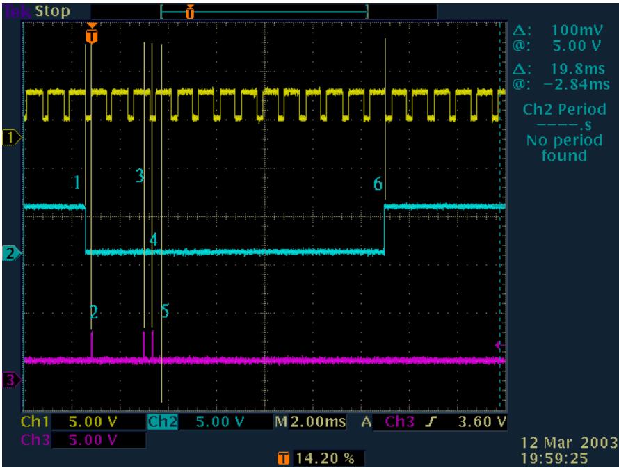
![| Channel | Voltage (mV) |\n|---------|--------------|\n| Ch1     | 100          |\n| Ch2     | 19.8         |\n| Ch3     | 14.20        |](.sscnet-series-manual-50-1h001-1020-204/0119ef88725e0d5e90387e13621cd39ebb88705a54a0f82490207d24c2a44405.jpg)

Figure 6-1: PCI-8372+ Single Motion Command Timing Chart

# Signal Channel:

▶ [1] DSP processing time synchronized with SSCNET cycle (low voltage level duration)
▶ DSP codes has two process: Synchronized and Non-Synchronized process, this channel displays the processing time of synchronized process.
[2] start\_tr\_move command processing time at host side (low voltage level duration)
▶ [3] DSP response time for Host motion command (high voltage level duration)

# Label number:

▶ (1)start\_tr\_move() command starts
▶ (1\~2) Trajectory calculation time on host
(2) Send motion-download command to DSP. DSP will take some time (the Peak) to transfer the trajectory data and set a “transferring done flag” for host.
▶ \*(2\~3) Host waits the “transferring done flag” and get a mutex from system for continue
▶ (3)Send motion-go command to DSP and DSP will take some time(the Peak) to set a “motion go” flag for DSP synchronized process
▶ (3\~4) DSP enter the synchronized process
▶ (4)DSP starts calculating first position for servo driver and put it on SSCNET data stream
▶ (4\~5) The position data is sent to servo driver through cable
▶ (5)Servo motor runs according to the position data
▶ \*\* (5\~6) Host start\_ta\_move() object is in ending process
▶ (6)start\_ta\_move function leaves

Note: \* Waiting mutex time is uncertain. It takes 2\~10ms in average.

\*\* C++ object dis-constructing time.

Conclusion: From Command Launched to Motor started takes about 3.5 SSCNET cycle

# 6.5 cPCI-8312H High Speed Link Initial Guide

cPCI-8312H has two master chips of High Speed Link on the board. So it has all the features of HSL just like PCI-7852. In this chapter, we will introduce how to to initial the HSL functions on this board.

# 1. MDSP\_Initial()

This function is not only for SSCNET but also initializing the board on Windows system. It will register the board's resources on system. The HSL functions are executable from this information only after the MDSP\_Initial() is successfully issued.

# 2. HSL\_Start() or HSL\_Auto\_Start()

This function will start to search all the modules on HSL network.

# 3. HSL\_Slave\_Live()

Use this function to check the status of searched HSL module

After these procedures, you can use all the functions of HSL. Please refer to HSL user's manual or module user guide for details.

# Warranty Policy

Thank you for choosing ADLINK. To understand your rights and enjoy all the after-sales services we offer, please read the following carefully.

1. Before using ADLINK's products please read the user manual and follow the instructions exactly. When sending in damaged products for repair, please attach an RMA application form which can be downloaded from: http://rma.adlinktech.com/policy/.

2. All ADLINK products come with a limited two-year warranty, one year for products bought in China:

The warranty period starts on the day the product is shipped from ADLINK's factory.
▶ Peripherals and third-party products not manufactured by ADLINK will be covered by the original manufacturers' warranty.
For products containing storage devices (hard drives, flash cards, etc.), please back up your data before sending them for repair. ADLINK is not responsible for any loss of data.
▶ Please ensure the use of properly licensed software with our systems. ADLINK does not condone the use of pirated software and will not service systems using such software. ADLINK will not be held legally responsible for products shipped with unlicensed software installed by the user.
For general repairs, please do not include peripheral accessories. If peripherals need to be included, be certain to specify which items you sent on the RMA Request & Confirmation Form. ADLINK is not responsible for items not listed on the RMA Request & Confirmation Form.

3. Our repair service is not covered by ADLINK's guarantee in the following situations:

▶ Damage caused by not following instructions in the User's Manual.
▶ Damage caused by carelessness on the user's part during product transportation.
▶ Damage caused by fire, earthquakes, floods, lightening, pollution, other acts of God, and/or incorrect usage of voltage transformers.
▶ Damage caused by unsuitable storage environments (i.e. high temperatures, high humidity, or volatile chemicals).
▶ Damage caused by leakage of battery fluid during or after change of batteries by customer/user.
▶ Damage from improper repair by unauthorized ADLINK technicians.
▶ Products with altered and/or damaged serial numbers are not entitled to our service.
▶ This warranty is not transferable or extendible.
▶ Other categories not protected under our warranty.

4. Customers are responsible for shipping costs to transport damaged products to our company or sales office.

5. To ensure the speed and quality of product repair, please download an RMA application form from our company website: http://rma.adlinktech.com/policy. Damaged products with attached RMA forms receive priority.

If you have any further questions, please email our FAE staff: service@adlinktech.com.
[🔗 Link to the original document](.sscnet-series-manual-50-1h001-1020-204/sscnet-series-manual-50-1h001-1020-204.pdf)